15 Accruals
In this chapter, we use Sloan (1996) to provide a focus for a study of accrual processes. We use simulation analysis to understand better accounting processes, with a particular focus on accruals, which for this chapter we define as the portion of earnings in excess of operating cash flows.1 We finish up the chapter with an examination of the so-called accrual anomaly.
The code in this chapter uses the packages listed below. For instructions on how to set up your computer to use the code found in this book, see Section 1.2. Quarto templates for the exercises below are available on GitHub.
15.1 Sloan (1996)
While we saw evidence in Chapter 14 that capital markets do not fully price earnings surprises, Sloan (1996) goes further and examines how capital markets price components of earnings. Sloan (1996) points out that a number of practitioners provide investment advice predicated on identifying firms whose earnings depend on accruals rather than cash flows. Such investment advice is based on a claimed tendency for capital markets to “fixate” on earnings and to fail to recognize differences in the properties of cash flow and accrual components of earnings. In some respects, Sloan (1996) provides a rigorous evaluation of such investment advice and the premises underlying it.
15.1.1 Discussion questions
The following discussion questions provide an approach to reading Sloan (1996). While one approach to reading a paper involves a careful reading from start to finish, a useful skill is being able to read a paper quickly with a focus on the empirical results and the hypotheses that these relate to.
Read the material preceding the formal statement of H1. What reasons for differential persistence of earnings components does Sloan (1996) offer? How important is it for these reasons to be correct in light of the empirical support for H1 provided in Table 3? How important is the empirical support for H1 to H2(i)?
Which hypothesis (if any) does Table 4 test? How would you interpret the results of Table 4 in words?
Which hypothesis (if any) does Table 5 test? How would you interpret the results of Table 5 in words?
Which hypothesis (if any) does Table 6 test? How would you interpret the results of Table 6 in words? There are similarities between the results of Table 6 of Sloan (1996) and the results in Bernard and Thomas (1989). Both involve forming portfolios of firms based on deciles of some variable (accruals in Sloan, 1996; earnings surprise in Bernard and Thomas, 1989) and examining how those portfolios perform subsequently. Apart from the measure used to form portfolios, what are the significant differences between the analyses in the two papers that you can think of looking at Table 6?
With which hypothesis (if any) is Figure 2 related? What does Figure 2 show according to Sloan (1996)?
With which hypothesis (if any) is Figure 3 related? What does Figure 3 show according to Sloan (1996)?
15.2 Measuring accruals
Hribar and Collins (2002) include a definition of accruals similar to that used in Sloan (1996). Referring to prior research, they state (2002, p. 10):
Specifically, accruals (\(\mathit{ACC}_{bs}\)) are typically calculated (firm and time subscripts omitted for convenience):
\[ \mathit{ACC}_{bs} = (\Delta \mathit{CA} - \Delta \mathit{CL} - \Delta \mathit{Cash} + \Delta \mathit{STDEBT} - \mathit{DEP} )\] where
- \(\Delta \mathit{CA}\) = the change in current assets during period \(t\) (Compustat #4)
- \(\Delta \mathit{CL}\) = the change in current liabilities during period \(t\) (Compustat #5)
- \(\Delta \mathit{Cash}\) = the change in cash and cash equivalents during period \(t\) (Compustat #1);
- \(\Delta \mathit{STDEBT}\) = the [change in] current maturities of long-term debt and other short-term debt included in current liabilities during period \(t\) (Compustat #34);
- and \(\Delta \mathit{DEP}\) = depreciation and amortization expense during period \(t\) (Compustat #14).
All variables are deflated by lagged total assets (\(\mathit{TA}_{t-1}\)) to control for scale differences.
The first thing you may ask is “what does (say) ‘Compustat #4’ mean?”. Prior to 2006, Compustat data items were referred to using numbers such as Compustat #4 or data4. So older papers may refer to such items. Fortunately, Wharton Research Data Services (WRDS) provides translation tables from these items to the current variables and relevant translations are provided in Table 15.1.
| Old item | Current item | Item description |
|---|---|---|
| #1 | che |
Cash and Short-Term Investments |
| #4 | act |
Current Assets—Total |
| #5 | lct |
Current Liabilities—Total |
| #14 | dp |
Depreciation and Amortization |
| #34 | dlc |
Debt in Current Liabilities—Total |
Hribar and Collins (2002) point out that calculating current accruals by subtracting the change in current liabilities from the change in noncash current assets is incorrect “because other non-operating events (e.g., mergers, divestitures) impact the current asset and liability accounts with no earnings impact.”
15.2.1 Discussion questions
In the equation above, why is \(\Delta \mathit{Cash}\) subtracted?
In the equation above, why is \(\Delta \mathit{STDEBT}\) added?
Is it true that mergers and divestitures have “no earnings impact”? Is the absence of earnings impact important to the estimation issue? Are there transactions that have no earnings impact, but do affect cash flow from operations?
Are there any differences between Hribar and Collins (2002) (\(\mathit{ACC}_{bs}\) above) and Sloan (1996) in their definitions of accruals? Which definition makes more sense to you? Why?
15.3 Simulation analysis
We now consider some simulation analysis. One reason for this analysis is to better understand the basis for H1 of Sloan (1996).
A second reason for conducting simulation analysis here is to illustrate the power it offers. In many contexts, derivation of the properties of estimators or understanding how phenomena interact is very complex. While many researchers rely on intuition to guide their analyses, such intuition can be unreliable. As an example, the idea that the “FM-NW” method provides standard errors robust to both time-series and cross-sectional dependence has strong intuitive appeal, but we saw in Chapter 5 that this intuition is simply wrong.
15.3.1 Vectors
In our simulation analysis, we make more extensive use of base R functionality than we have in prior chapters. Chapter 28 of R for Data Science—“A field guide to base R”—provides material that might be helpful if code in the next section is unclear. Here we are simulating the cash flows and accounting for a simple firm that buys goods for cash and sells them on account after adding a mark-up.
15.3.2 Simulation function
As we have seen before, it is often a good coding practice to use functions liberally in analysis.2 In this case, we embed the core of the simulation in a function.
The simulation function get_data() below generates a time-series of data for a single “firm” and accepts two arguments. The first argument to get_data() is add_perc, which has a default value of 0.03. The value of add_perc drives the amount of allowance for doubtful debts. The second argument is n_years, which has a default value of 20. The value of n_years drives the number of years of data generated by the simulation.
The simulation generates various cash flows and the financial statements to represent them. The main driver of the model is sales, which follows an autoregressive process. Denoting sales in period \(t\) as \(S_t\), we have
\[ S_{t} - \overline{S} = \rho (S_{t-1} - \overline{S}) + \epsilon_t \] where \(\rho \in (0, 1)\) and \(\epsilon_t \sim N(0, \sigma^2)\).
Sales then drives both cost of goods sold, which are assumed to require cash outlays in the period of sale, and accounts receivable, as all sales are assumed to be on account. The model also addresses collections, write-offs, and dividends. There are no inventories in our model.
In the simulation function, we use “base R” functionality to a fair degree. Rather than using mutate() to generate variables, we refer to variables using $ notation, which returns the variable as a vector. For example df |> select(ni) returns a data frame with a single column. In contrast, df$ni gets the same underlying data, but as a vector. To calculate shareholders’ equity (se), we set the initial (\(t=0\)) value to beg_se. Then we calculate the ending balance of shareholders’ equity as beginning shareholders’ equity plus net income minus dividends.
get_data <- function(add_perc = 0.03, n_years = 20) {

    # Parameters
    add_true <- 0.03
    gross_margin <- 0.8
    beg_cash <- beg_se <- 1500
    div_payout <- 1
    mean_sale <- 1000
    sd_sale <- 100
    rho <- 0.9

    # Generate sales as an AR(1) process around mean_sale
    sale_err <- rnorm(n_years, sd = sd_sale)
    sales <- vector("double", n_years)
    sales[1] <- mean_sale + sale_err[1]
    for (i in 2:n_years) {
      sales[i] = mean_sale +  rho * (sales[i-1] - mean_sale) + sale_err[i]
    }

    # Combine data so far into a data frame;
    # add slots for variables to come
    df <- tibble(year = 1:n_years,
                 add_perc = add_perc,
                 sales,
                 writeoffs = NA, collect = NA,
                 div = NA, se = NA, ni = NA,
                 bde = NA, cash = NA)

    # All sales at the same margin
    df$cogs <- (1 - gross_margin) * df$sales

    # All sales are on credit;
    # collections/write-offs occur in next period
    df$ar <- df$sales

    # Allowance for doubtful debts
    df$add <- add_perc * df$sales

    # Calculate year-1 values
    df$writeoffs[1] <- 0
    df$collect[1] <- 0
    df$bde[1] <- df$add[1]
    df$ni[1] <- df$sales[1] - df$cogs[1] - df$bde[1]
    df$div[1] <- df$ni[1] * div_payout
    df$cash[1] <- beg_cash + df$collect[1] - df$cogs[1] - df$div[1]
    df$se[1] <- beg_se + df$ni[1] - df$div[1]

    # Loop through years from 2 to n_years
    for (i in 2:n_years) {
      df$writeoffs[i] <- add_true * df$ar[i-1]
      df$collect[i] <- (1 - add_true) * df$ar[i-1]
      df$bde[i] = df$add[i] - df$add[i-1] + df$writeoffs[i]
      df$ni[i] <- df$sales[i] - df$cogs[i] - df$bde[i]
      df$div[i] <- df$ni[i] * div_payout
      df$cash[i] <- df$cash[i-1] + df$collect[i] - df$cogs[i] - df$div[i]
      df$se[i] <- df$se[i-1] + df$ni[i] - df$ni[i]
    }

    df
}
To understand a function like this, it can be helpful to set values for the arguments (e.g., add_perc <- 0.03; n_years <- 20) and step through the lines of code one by one, intermittently inspecting the content of variables such as df as you do so.3
Let’s generate 1000 years of data.
set.seed(2021)
df_1000 <- get_data(n_years = 1000)
The first 20 years are shown in Figure 15.1.
df_1000 |>
  filter(year <= 20) |>
  ggplot(aes(x = year)) +
  geom_line(aes(y = sales), colour = "red") +
  geom_line(aes(y = mean(sales)), colour = "blue")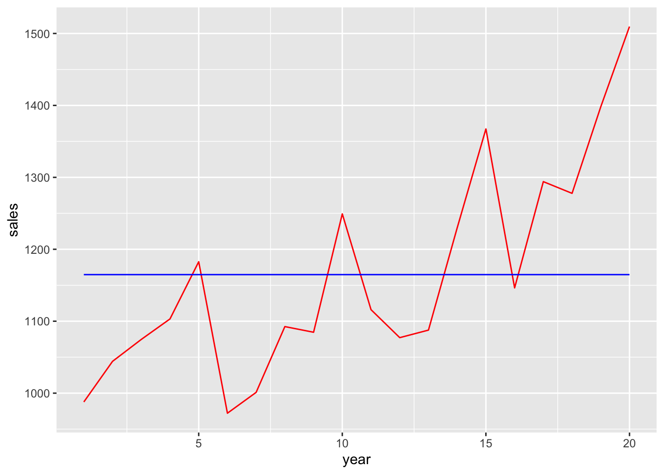
Now, let’s generate 5,000 random values for the add_perc parameter that we can use to generate simulated data.
add_percs <- runif(n = 5000, min = 0.01, max = 0.05)We will generate simulated data for each value add_percs and store these data in a list called res_list.
set.seed(2021)

res_list <-
  map(add_percs, get_data) |>
  system_time()
user system elapsed
16.303 0.057 16.535 While production of res_list takes just a few seconds, because each iteration of get_data() is independent of the others, we could use the future package and plan(multisession) to do it even more quickly.
plan(multisession)

res_list <-
  future_map(add_percs, get_data,
             .options = furrr_options(seed = 2021)) |>
  system_time()
user system elapsed
0.467 0.024 4.270 We then make two data frames. The first data frame (res_df) stores all the data in a single data frame using the field id to distinguish one simulation run from another. These runs might be considered as “firms” with each run being independent of the other.
res_df <- list_rbind(res_list, names_to = "id")To make it easier to compile results, we create get_coefs(), which calculates persistence as the coefficient in a regression of income on its lagged value—a specification similar to that in Sloan (1996)—and returns that value.
We apply get_coefs() to res_list and store the results in the second data frame, results.
results <-
  res_list |>
  map(get_coefs) |>
  list_rbind(names_to = "id")
We plot the estimated persistence value against the assumed value for add_perc in Figure 15.2.
results |>
  ggplot(aes(x = add_perc, y = persistence)) +
  geom_point()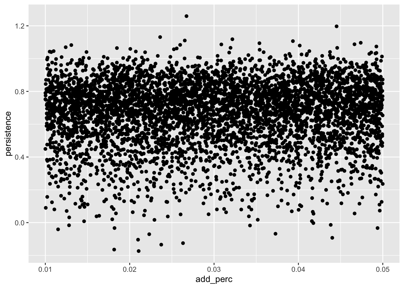
add_perc
15.3.3 Exercises
When generating simulated financial statement data, it is generally important to ensure that the generated data meet some basic requirements. What is one fundamental relation that we expect to hold for these data? Does it hold for the data in
df_1000?Calculate values for cash flows from operating activities and cash flows from financing activities. (Treat payment of dividends as a financing activity. Hint: You may find it easier to use the direct method to calculate cash flows from operating activities.) Does the cash flow statement articulate as it should?
How evident are the details of the underlying process generating sales from Figure 15.1? Does looking at more data help? (Obviously, having a thousand years of data on a firm with a stationary process is not common.)
What is the “correct” value of
add_percthat should be used? Using the plot fromresultsabove, what is the relation between values of departing from that value and persistence? Does this agree with your intuition? What’s going on? What aspects of theadd_perc-related accounting seem unrealistic? (Hint: It may help to use variant of the following codeset.seed(2021); get_data(0.03)for various values in place of0.03and to examine how the earnings process is affected.)Does the simulation analysis speak to the underlying rationale for H1 of Sloan (1996)? If so, why? If not, what might be missing from the analysis? How might we modify the simulation to incorporate the missing elements?
15.4 Replicating Sloan (1996)
To better understand some elements of the empirical analysis of Sloan (1996), we conduct a replication analysis.
We start by collating the data. We first connect to the tables we will use in our analysis.
db <- dbConnect(duckdb::duckdb())

funda <- load_parquet(db, schema = "comp", table = "funda")
company <- load_parquet(db, schema = "comp", table = "company")
ccmxpf_lnkhist <- load_parquet(db, schema = "crsp", table = "ccmxpf_lnkhist")
msf <- load_parquet(db, schema = "crsp", table = "msf")
We then make a subset of comp.funda, add SIC data from comp.company, and call the result funda_mod. We construct SIC codes using sich, which provides the “historical” SIC code (sich), where available, but we use the “header” SIC code (sic) found on comp.company when sich is unavailable.4 For some reason, sic is a character variable on comp.company and sich is an integer on comp.funda. So, we convert sic to an integer before merging the two tables here.
We next apply the same sample selection criteria as Sloan (1996). We focus on NYSE and AMEX firm-years (i.e., ones with exchg equal to 11 and 12, respectively) and years between 1962 and 1991.
Sloan (1996, p. 293) suggests that “the financial statement data required to compute operating accruals are not available … on Compustat for banks, life insurance or property and casualty companies.” However, it is not clear if these firms are explicitly excluded (e.g., by filtering on SIC codes) or implicitly excluded by simply requiring that data for calculating accruals be available. As such, we retain these firms and merely create a related indicator variable (finance).
The next step is to create variables to reflect changes in key variables. We can use lag() to do this.5
acc_data_raw <-
  funda_mod |>
  filter(!is.na(at),
         pddur == 12,
         exchg %in% c(11L, 12L)) |>
  mutate(finance = between(sic, 6000, 6999),
         across(c(che, dlc, txp), \(x) coalesce(x, 0))) |>
  group_by(gvkey) |>
  window_order(datadate) |>
  mutate(avg_at = (at + lag(at)) / 2,
         d_ca = act - lag(act),
         d_cash = che - lag(che),
         d_cl = lct - lag(lct),
         d_std = dlc - lag(dlc),
         d_tp = txp - lag(txp)) |>
  select(gvkey, datadate, fyear, avg_at, at, oiadp, dp, finance,
         starts_with("d_"), sic, pddur) |>
  mutate(acc_raw =  (d_ca - d_cash) - (d_cl - d_std - d_tp) - dp) |>
  ungroup() |>
  filter(between(fyear, 1962, 1991),
         avg_at > 0)
The final step in our data preparation calculates the core variables earn, acc, and cfo according to the definitions found in Sloan (1996), creates a variable to store the leading value of earn (using the lead() function, which is a window function that complements the lag() function we used above), creates deciles for acc, earn, cfo, and lead_earn, creates a two-digit SIC code, and finally filters out finance firms and observations without values for acc.
acc_data <-
  acc_data_raw |>
  mutate(earn = oiadp / avg_at,
         acc = acc_raw / avg_at,
         cfo = earn - acc) |>
  group_by(gvkey) |>
  window_order(datadate) |>
  mutate(lead_earn = lead(earn)) |>
  ungroup() |>
  collect() |>
  mutate(acc_decile = ntile(acc, 10),
         earn_decile = ntile(earn, 10),
         cfo_decile = ntile(cfo, 10),
         lead_earn_decile = ntile(lead_earn, 10),
         sic2 = str_sub(as.character(sic), 1, 2)) |>
  filter(!finance, !is.na(acc))
The next step is to collect data on stock returns for each firm-year. We use ccm_link, which we saw in Chapter 7, to link GVKEYs (Compustat) to PERMNOs (CRSP).
Following Sloan (1996), we link (gvkey, datadate) combinations with permnos and a date range for the twelve-month period beginning four months after the end of the fiscal period.
crsp_link <-
  acc_data_raw |>
  select(gvkey, datadate) |>
  inner_join(ccm_link,
             join_by(gvkey, between(datadate, linkdt, linkenddt))) |>
  select(gvkey, datadate, permno) |>
  mutate(start_month = as.Date(floor_date(datadate + months(4L), "month")),
         end_month = as.Date(floor_date(datadate + months(16L) - days(1L),
                                        "month")),
         month = floor_date(datadate, 'month'))
We then calculate compounded returns over this window for each (gvkey, datadate, permno) combination.
Table 4 of Sloan (1996, p. 304) uses abnormal returns, which are “computed by taking the raw buy-hold return … and subtracting the buy-hold return of a size-matched, value-weighted portfolio of firms. The size portfolios are based on market value of equity deciles of NYSE and AMEX firms.” We obtained the returns of individual firms above, but need to collect data on size portfolios, both the returns for each portfolio and the market capitalization cut-offs.
Data for size portfolios come from Ken French’s website, as we saw in Chapter 11. Code like that used in Chapter 11 is included in the farr package in two functions: get_size_rets_monthly() and get_me_breakpoints().
size_rets <- get_size_rets_monthly()
size_rets
# A tibble: 11,690 × 4
month decile ew_ret vw_ret
<date> <int> <dbl> <dbl>
1 1926-07-01 1 -0.0142 -0.0012
2 1926-07-01 2 0.0029 0.0052
3 1926-07-01 3 -0.0015 -0.0005
4 1926-07-01 4 0.0088 0.0082
5 1926-07-01 5 0.0145 0.0139
6 1926-07-01 6 0.0185 0.0189
7 1926-07-01 7 0.0163 0.0162
8 1926-07-01 8 0.0138 0.0129
9 1926-07-01 9 0.0338 0.0353
10 1926-07-01 10 0.0329 0.0371
# ℹ 11,680 more rowsThe table returned by get_size_rets_monthly() has four columns, including two measures of returns: one based on equal-weighted portfolios (ew_ret) and one based on value-weighted portfolios (vw_ret). Like Sloan (1996), we use vw_ret.
me_breakpoints <- get_me_breakpoints()
me_breakpoints
# A tibble: 11,760 × 4
month decile me_min me_max
<date> <int> <dbl> <dbl>
1 1925-12-01 1 0 2.38
2 1925-12-01 2 2.38 4.95
3 1925-12-01 3 4.95 7.4
4 1925-12-01 4 7.4 10.8
5 1925-12-01 5 10.8 15.6
6 1925-12-01 6 15.6 22.9
7 1925-12-01 7 22.9 38.4
8 1925-12-01 8 38.4 65.8
9 1925-12-01 9 65.8 142.
10 1925-12-01 10 142. Inf
# ℹ 11,750 more rowsThe table returned by get_me_breakpoints() identifies the size decile (decile) to which firms with market capitalization between me_min and me_max in a given month should be assigned.
To join CRSP with crsp_link, we construct the variable month for each value of date on crsp.msf. This prevents non-matches due to non-alignment of datadate values with date values on crsp.msf.
crsp_dates <-
  msf |>
  distinct(date) |>
  mutate(month = floor_date(date, 'month'))
The following code assigns firm-years (i.e., (permno, datadate) combinations) to size deciles according to market capitalization and size cut-offs applicable during the month of datadate.
me_values <-
  crsp_link |>
  inner_join(crsp_dates, by = "month") |>
  inner_join(msf, by = c("permno", "date")) |>
  mutate(mktcap = abs(prc) * shrout / 1000) |>
  select(permno, datadate, month, mktcap) |>
  collect()

me_decile_assignments <-
  me_breakpoints |>
  inner_join(me_values,
             join_by(month, me_min <= mktcap, me_max > mktcap)) |>
  select(permno, datadate, decile)
For each datadate and size decile, the following code calculates the cumulative returns over the twelve-month period beginning four months after datadate.
cum_size_rets <-
  me_decile_assignments |>
  select(datadate, decile) |>
  distinct() |>
  mutate(start_month = datadate + months(4),
         end_month =  datadate + months(16)) |>
  inner_join(size_rets,
             join_by(decile, start_month <= month, end_month >= month)) |>
  group_by(datadate, decile) |>
  summarize(ew_ret = exp(sum(log(1 + ew_ret), na.rm = TRUE)) - 1,
            vw_ret = exp(sum(log(1 + vw_ret), na.rm = TRUE)) - 1,
            n_size_months = n(),
            .groups = "drop")
Now we have the data we need to calculate size-adjusted returns. We simply combine crsp_data with me_decile_assignments and then with cum_size_rets and calculate size_adj_ret as a simple difference.
size_adj_rets <-
  crsp_data |>
  inner_join(me_decile_assignments, by = c("permno", "datadate")) |>
  inner_join(cum_size_rets, by = c("datadate", "decile")) |>
  mutate(size_adj_ret = ret - vw_ret) |>
  select(gvkey, datadate, size_adj_ret, n_months, n_size_months)
For our regression analysis, we simply join our processed data from Compustat (acc_data) with our new data on size-adjusted returns (size_adj_rets).
reg_data <-
  acc_data |>
  inner_join(size_adj_rets, by = c("gvkey", "datadate"))
Before running regression analyses, it is important to examine our data. One useful benchmark is the set of descriptive statistics reported in Table 1 of Sloan (1996). Some degree of assurance is provided by the similar of the values seen in Table 15.2 with those reported in Sloan (1996).
reg_data |>
  group_by(acc_decile) |>
summarize(across(c(acc, earn, cfo), \(x) mean(x, na.rm = TRUE)))| acc_decile | acc | earn | cfo |
|---|---|---|---|
| 1 | -0.175 | 0.035 | 0.211 |
| 2 | -0.087 | 0.095 | 0.182 |
| 3 | -0.061 | 0.104 | 0.165 |
| 4 | -0.044 | 0.111 | 0.155 |
| 5 | -0.030 | 0.118 | 0.148 |
| 6 | -0.017 | 0.118 | 0.135 |
| 7 | -0.001 | 0.127 | 0.128 |
| 8 | 0.023 | 0.135 | 0.113 |
| 9 | 0.060 | 0.142 | 0.082 |
| 10 | 0.172 | 0.154 | -0.018 |
15.4.1 Table 2 of Sloan (1996)
Having done a very basic check of our data, we can create analogues of some of the regression analyses found in Sloan (1996).
The output shown in Table 15.3 parallels the “pooled” results in Table 2 of Sloan (1996).
fms <- list(lm(lead_earn ~ earn, data = reg_data),
            lm(lead_earn_decile ~ earn_decile, data = reg_data))

modelsummary(fms,
             estimate = "{estimate}{stars}",
             gof_map = c("nobs", "r.squared"),
stars = c('*' = .1, '**' = 0.05, '***' = .01))| (1) | (2) | |
|---|---|---|
| (Intercept) | 0.030*** | 1.396*** |
| (0.001) | (0.039) | |
| earn | 0.704*** | |
| (0.005) | ||
| earn_decile | 0.749*** | |
| (0.006) | ||
| Num.Obs. | 12877 | 12877 |
| R2 | 0.607 | 0.553 |
To produce “industry level” analysis like that in Table 2 of Sloan (1996), we create run_table_ind(), a small function to produce regression coefficients by industry. As seen in Chapter 14, we use !! to distinguish the value sic2 supplied to the function from the variable sic2 found in reg_data.6
The function stats_for_table() compiles descriptive statistics.
Finally, summ_for_table() calls run_table_ind() and stats_for_table() and produces a summary table.
summ_for_table <- function(lhs = "lead_earn", rhs = "earn") {
  reg_data |>
    distinct(sic2) |>
    pull() |>
    map(run_table_ind, lhs = lhs, rhs = rhs) |>
    list_rbind() |>
    select(-sic2) |>
    map(stats_for_table) |>
    list_rbind(names_to = "term")
}
Tables 15.4 and 15.5 parallel the “industry level” results reported in Table 2 of Sloan (1996).
summ_for_table(lhs = "lead_earn", rhs = "earn")| term | mean | q1 | median | q3 |
|---|---|---|---|---|
| (Intercept) | 0.026 | 0.012 | 0.026 | 0.036 |
| earn | 0.664 | 0.611 | 0.697 | 0.815 |
summ_for_table(lhs = "lead_earn_decile", rhs = "earn_decile")| term | mean | q1 | median | q3 |
|---|---|---|---|---|
| (Intercept) | 1.612 | 0.937 | 1.257 | 1.745 |
| earn_decile | 0.670 | 0.649 | 0.739 | 0.819 |
Our results thus far might be described as “qualitatively similar” to those in Table 2 of Sloan (1996). The main difference may be in the magnitude of the pooled coefficient on earn in the regression with lead_earn as the dependent variable. Table 2 of Sloan (1996) reports a coefficient of 0.841, notably higher than the mean coefficient from the industry-level regressions (0.773). In contrast, the mean coefficients in our pooled and industry-level analyses are much closer to each other.
15.4.2 Table 3 of Sloan (1996)
In Table 3, Sloan (1996) decomposes the right-hand side variables from Table 15.3 into accrual and cash-flow components. We replicate these analyses in Table 15.6.
fms <- list(lm(lead_earn ~ acc + cfo, data = reg_data),
            lm(lead_earn_decile ~ acc_decile + cfo_decile, data = reg_data))

modelsummary(fms,
             estimate = "{estimate}{stars}",
             gof_map = c("nobs", "r.squared"),
stars = c('*' = .1, '**' = 0.05, '***' = .01))| (1) | (2) | |
|---|---|---|
| (Intercept) | 0.028*** | -1.312*** |
| (0.001) | (0.073) | |
| acc | 0.640*** | |
| (0.007) | ||
| cfo | 0.723*** | |
| (0.005) | ||
| acc_decile | 0.534*** | |
| (0.007) | ||
| cfo_decile | 0.760*** | |
| (0.007) | ||
| Num.Obs. | 12877 | 12877 |
| R2 | 0.613 | 0.470 |
Tables 15.7 and 15.8 parallel the “industry level” results reported in Table 3 of Sloan (1996). Again we have “qualitatively similar” results to those found in Sloan (1996).
summ_for_table(lhs = "lead_earn", rhs = "acc + cfo")| term | mean | q1 | median | q3 |
|---|---|---|---|---|
| (Intercept) | 0.025 | 0.010 | 0.024 | 0.031 |
| acc | 0.671 | 0.589 | 0.667 | 0.766 |
| cfo | 0.714 | 0.651 | 0.723 | 0.828 |
summ_for_table(lhs = "lead_earn_decile", rhs = "acc_decile + cfo_decile")| term | mean | q1 | median | q3 |
|---|---|---|---|---|
| (Intercept) | -0.880 | -2.029 | -1.284 | -0.610 |
| acc_decile | 0.485 | 0.438 | 0.520 | 0.598 |
| cfo_decile | 0.697 | 0.672 | 0.735 | 0.845 |
15.4.3 Pricing of earnings components
An element of the analysis reported in Table 5 of Sloan (1996) regresses abnormal returns on contemporaneous earnings and components of lagged earnings and we do likewise.
Table 15.9 provides results from this regression.
modelsummary(mms,
             estimate = "{estimate}{stars}",
             gof_map = c("nobs", "r.squared"),
stars = c('*' = .1, '**' = 0.05, '***' = .01))| (1) | (2) | |
|---|---|---|
| (Intercept) | -0.027*** | 0.186*** |
| (0.006) | (0.018) | |
| lead_earn | 2.538*** | |
| (0.061) | ||
| acc | -1.961*** | |
| (0.062) | ||
| cfo | -1.826*** | |
| (0.057) | ||
| lead_earn_decile | 0.082*** | |
| (0.002) | ||
| acc_decile | -0.055*** | |
| (0.002) | ||
| cfo_decile | -0.056*** | |
| (0.002) | ||
| Num.Obs. | 12867 | 12867 |
| R2 | 0.124 | 0.109 |
In the notation of Sloan (1996), the coefficient on acc can be expressed as \(- \beta \gamma^{*}_1\), which is minus one times the product of \(\beta\), the coefficient on lead_earn (i.e., earnings roughly contemporaneous with size_adj_ret), and \(\gamma^{*}_1\), the implied market coefficient on accruals.
With estimates of \(\hat{\beta} = 2.538\) and \(\widehat{\beta \gamma^{*}_1} = 1.961\), we have an implied estimate of \(\hat{\gamma}^{*}_1 = 0.7726.\)
This estimate \(\hat{\gamma}^{*}_1 = 0.7726\) is higher than the estimate of \(\hat{\gamma}_1 = 0.6399\). But can we conclude that the difference between these two coefficients is statistically significant?
One approach to this question would be to evaluate whether \(\widehat{\beta \gamma^{*}_1} = 1.961\) as estimated from the market regression is statistically different from the value implied by \(\hat{\beta} \times \hat{\gamma_1} = 2.538 \times 0.6399 = 1.624\).
However, as pointed out by Mishkin (1983), this procedure “implicitly assumes that there is no uncertainty in the estimate of \(\hat{\gamma_1}\). This results in inconsistent estimates of the standard errors of the parameters and hence test statistics that do not have the assumed F distribution. This can lead to inappropriate inference ….”7
Given the issue of “inappropriate inference” described above, Mishkin (1983) uses “iterative weighted non-linear least squares” (Sloan, 1996, p. 302) to estimate a system of equations and then calculates an F-statistic based on comparison of goodness-of-fit of an unconstrained system of equations with that of a constrained system of equations (i.e., one in which \(\gamma\) is constrained equal in both equations). While Sloan (1996) uses this “Mishkin (1983)” test in his analysis reported in Tables 4 and 5, this approach involves significant complexity.8
Fortunately, Abel and Mishkin (1983) suggest a simpler approach that they show is asymptotically equivalent to the Mishkin test. The intuition for this approach is that if components of lagged earnings (accruals and cash flows) are mispriced in a way that predicts stock returns, then this should be apparent from a regression of stock returns on those lagged earnings components. Kraft et al. (2007) provide additional discussion of the Mishkin test and the approach used by Abel and Mishkin (1983).9 In effect, this allows us to skip the “middleman” of contemporaneous earnings in the regression analysis.
The regression results in Table 15.10 come from applying the approach suggested by Abel and Mishkin (1983).
eff <- list(lm(size_adj_ret ~ acc + cfo, data = reg_data),
            lm(size_adj_ret ~ acc_decile + cfo_decile, data = reg_data))

modelsummary(eff,
             estimate = "{estimate}{stars}",
             gof_map = c("nobs", "r.squared"),
stars = c('*' = .1, '**' = 0.05, '***' = .01))| (1) | (2) | |
|---|---|---|
| (Intercept) | 0.041*** | 0.078*** |
| (0.006) | (0.018) | |
| acc | -0.327*** | |
| (0.049) | ||
| cfo | 0.038 | |
| (0.037) | ||
| acc_decile | -0.011*** | |
| (0.002) | ||
| cfo_decile | 0.006*** | |
| (0.002) | ||
| Num.Obs. | 13798 | 13798 |
| R2 | 0.005 | 0.007 |
From Table 15.10, we see that lagged accruals are negatively associated with abnormal returns. This result is consistent with the market overpricing accruals because it assumes a level of persistence that is too high.
15.4.4 Exercises
In creating
acc_data_raw, we usedcoalesce()to set the value of certain variables to zero when missing on Compustat. Does this seem appropriate here? Are the issues similar to those observed with regard to R&D in Chapter 8? It may be helpful to find some observations from recent years where this use of thecoalesce()function has an effect and think about the issues in context of financial statements for those firm-years.Can you reconcile the results from the Abel and Mishkin (1983) test with those from the previous regressions? (Hint: Pay attention to sample composition; you may need to tweak these regressions.)
The equations estimated in Table 5 of Sloan (1996) could be viewed as a structural (causal) model. Can you represent this model using a causal diagram? In light of the apparent econometric equivalence between that structural model and the estimation approach used in Abel and Mishkin (1983), how might the coefficients from the structural model be recovered from the latter approach?
A critique of Sloan (1996) made by Kraft et al. (2007) is that the coefficients may be biased due to omitted variables. This critique implies a causal interpretation of the coefficients in Sloan (1996). How might the critique of Kraft et al. (2007) be represented on the causal diagrams above? How persuasive do you find the critique of Kraft et al. (2007) to be?
Apart from the different data sources used, another difference between the simulation analysis earlier in this chapter and the regression analysis in Table 3 of Sloan (1996) is the regression model used. Modify the code below to incorporate the appropriate formulas for cash flow from operating activities (
cfo) and accruals (acc). Then replicate the pooled analysis of Panel A of Table 3 of Sloan (1996) using the resultingsim_reg_datadata frame. What do you observe?
sim_reg_data <-
  res_df |>
  mutate(cfo = [PUT CALC HERE], acc = [PUT CALC HERE]) |>
  group_by(id) |>
  arrange(id, year) |>
  mutate(lag_cfo = lag(cfo),
         lag_acc = lag(acc)) |>
ungroup()- Which hypothesis does Figure 1 of Sloan (1996) relate to? What aspects of the plot make it easier or more difficult to interpret the results? The following code replicates a version of Figure 1 from Sloan (1996) using our simulated data. On the basis of Figures 15.3–15.5 and the arguments given in Sloan (1996), is H1 true in our simulated data? Given the other analysis above, is H1 true in our simulated data?
The following code produces Figure 15.3:
reg_data_deciles |>
  filter(ni_decile %in% c(1, 10)) |>
  mutate(ni_decile = as.factor(ni_decile),
         event_year = year - year_of_event) |>
  group_by(ni_decile, year) |>
  summarize(ni = mean(ni, na.rm = TRUE), .groups = "drop") |>
  ggplot(aes(x = year, y = ni, group= ni_decile, color = ni_decile)) +
  geom_line()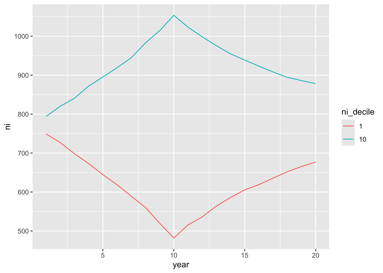
The following code produces Figure 15.4:
reg_data_deciles |>
  filter(cfo_decile %in% c(1, 10)) |>
  mutate(cfo_decile = as.factor(cfo_decile),
         event_year = year - year_of_event) |>
  group_by(cfo_decile, year) |>
  summarize(ni = mean(ni, na.rm = TRUE), .groups = "drop") |>
  ggplot(aes(x = year, y = ni, group = cfo_decile, color = cfo_decile)) +
  geom_line()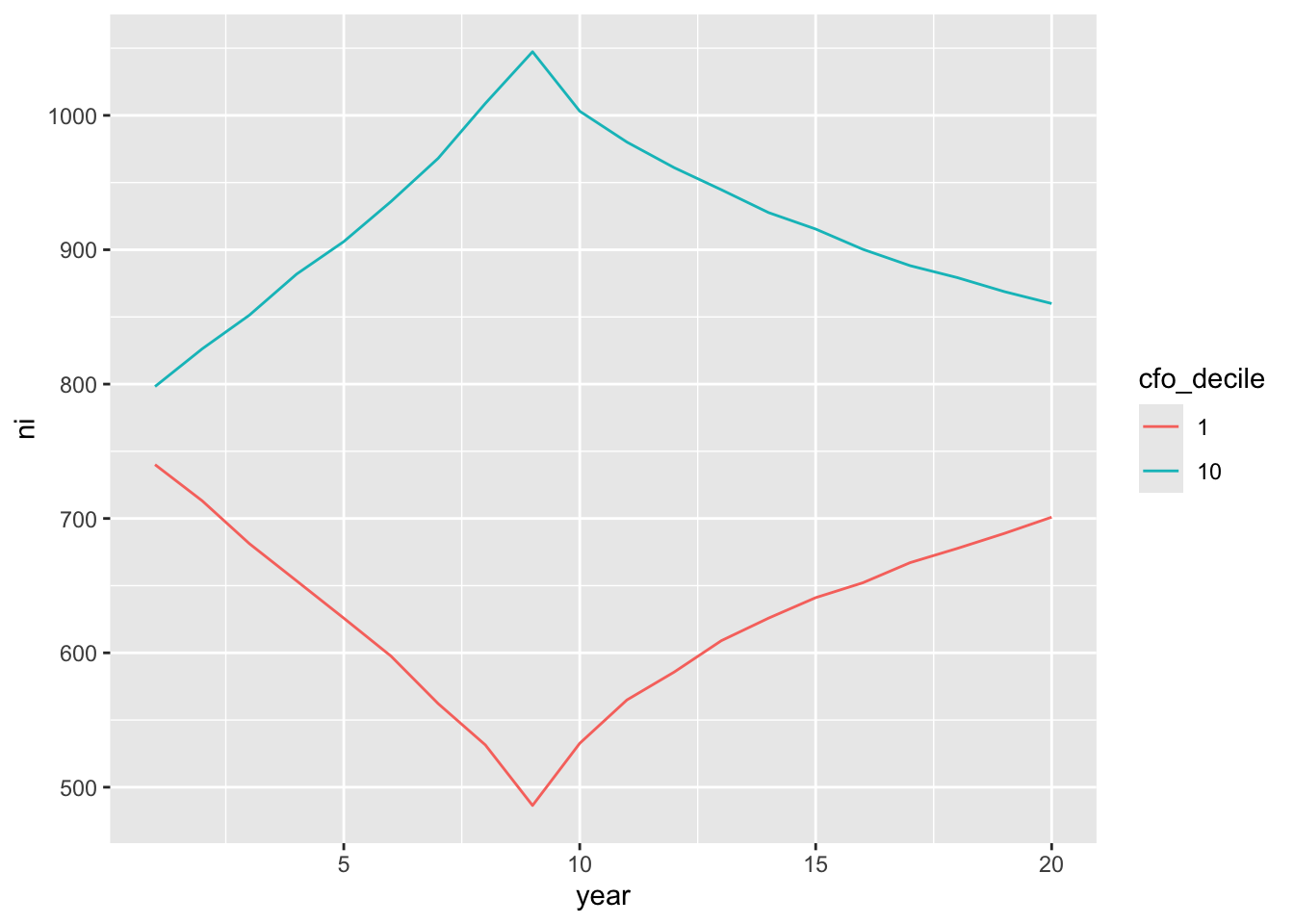
The following code produces Figure 15.5:
reg_data_deciles |>
  filter(acc_decile %in% c(1, 10)) |>
  mutate(acc_decile = as.factor(acc_decile),
         event_year = year - year_of_event) |>
  group_by(acc_decile, year) |>
  summarize(ni = mean(ni, na.rm = TRUE), .groups = "drop") |>
  ggplot(aes(x = year, y = ni, group = acc_decile, color = acc_decile)) +
  geom_line()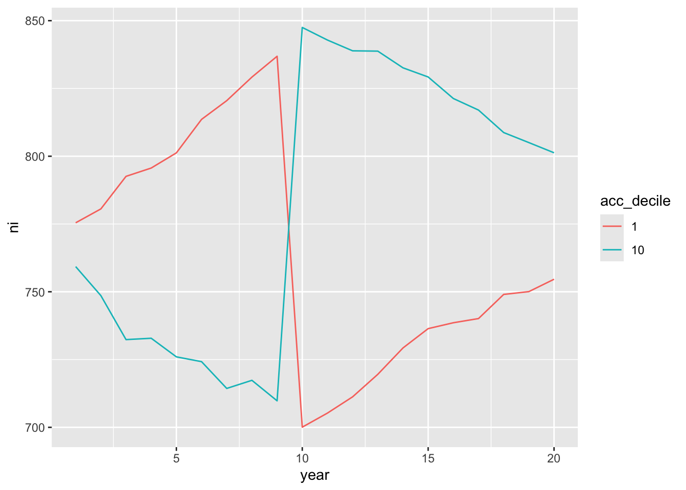
15.5 Accrual anomaly
Table 6 of Sloan (1996) provides evidence that the market’s apparent mispricing of accruals implies trading strategies that give rise to abnormal returns. Such strategies are generally termed anomalies because they seem inconsistent with the efficient markets hypothesis (see Section 10.1). Fama and French (2008, p. 1653) define anomalies as “patterns in average stock returns that … are not explained by the Capital Asset Pricing Model (CAPM).” Implicit in the Fama and French (2008) seems to be the notion that the CAPM is the true model of market risk and a general version of the definition of Fama and French (2008) would replace the CAPM with the posited true model of market risk. Dechow et al. (2011, p. 23) argue that “the accrual anomaly is not really an anomaly at all. In fact, the original research documenting the accrual anomaly predicted that it would be there. The term anomaly is usually reserved for behavior that deviates from existing theories, but when Sloan (1996) first documented the accrual anomaly, he was testing a well-known theory and found that it was supported.”
While Table 6 provides portfolio returns for years \(t+1\), \(t+2\), and \(t+3\), we only collected returns for year \(t+1\) in the steps above. Therefore, Table 15.11 only replicates the first column of Table 6 of Sloan (1996).
fm <-
  reg_data |>
  group_by(fyear, acc_decile) |>
  summarize(size_adj_ret = mean(size_adj_ret, na.rm = TRUE),
            .groups = "drop") |>
  mutate(acc_decile = as.factor(acc_decile)) |>
  lm(size_adj_ret ~ acc_decile - 1, data = _)

modelsummary(fm,
             estimate = "{estimate}{stars}",
             gof_map = c("nobs", "r.squared"),
stars = c('*' = .1, '**' = 0.05, '***' = .01))| (1) | |
|---|---|
| acc_decile1 | 0.120*** |
| (0.020) | |
| acc_decile2 | 0.109*** |
| (0.020) | |
| acc_decile3 | 0.042** |
| (0.020) | |
| acc_decile4 | 0.058*** |
| (0.020) | |
| acc_decile5 | 0.067*** |
| (0.020) | |
| acc_decile6 | 0.042** |
| (0.020) | |
| acc_decile7 | 0.025 |
| (0.020) | |
| acc_decile8 | 0.034* |
| (0.020) | |
| acc_decile9 | -0.003 |
| (0.020) | |
| acc_decile10 | -0.012 |
| (0.020) | |
| Num.Obs. | 300 |
| R2 | 0.255 |
hedge_ret <- fm$coefficients["acc_decile1"] - fm$coefficients["acc_decile10"]
p_val <- linearHypothesis(fm, "acc_decile1 = acc_decile10")$`Pr(>F)`[2]
The hedge portfolio return (hedge_ret) is 0.1322 with a p-value of 4.4e-06 (p_val).
15.5.1 Discussion questions
In estimating the hedge portfolio regression, we included a line
summarize(size_adj_ret = mean(size_adj_ret)). Why is this step important?Green et al. (2011) say “the simplicity of the accruals strategy and the size of the returns it generates have led some scholars to conclude that the anomaly is illusory. For example, Khan (2008) and Wu et al. (2010) argue that the anomaly can be explained by a mis-specified risk model and the q-theory of time-varying discount rates, respectively; Desai et al. (2004) conclude that the anomaly is deceptive because it is subsumed by a different strategy; Kraft et al. (2006) attribute it to outliers and look-ahead biases; Ng (2005) proposes that the anomaly’s abnormal returns are compensation for high exposure to bankruptcy risk; and Zach (2006) argues that there are firm characteristics correlated with accruals that cause the return pattern.” Looking at Sloan (1996), but without necessarily looking at each of the papers above, what evidence in Sloan (1996) seems inconsistent with the claims made by each paper above? Which do you think you would need to look more closely at the paper to understand? What evidence do you think Zach (2006) would need to provide to support the claim of an alternative “cause”?
Do Green et al. (2011) address the alternative explanations advanced in the quote in Q1 above? Do you think that they need to do so?
How persuasive do you find the evidence regarding the role of hedge funds provided by Green et al. (2011)?
Xie (2001) (p. 360) says that “for firm-years prior to 1988 when Compustat item #308 is unavailable, I estimate \(\textit{CFO}_t\) as follows …”. Why would item #308 be unavailable prior to 1988? What is the equivalent to #308 in Compustat today?
Study the empirical model on p. 361 of Xie (2001), which is labelled equation (1). (This is the much-used “Jones model” from Jones (1991), which we examine in Chapter 16.) What are the assumptions implicit in this model and the labelling of the residual as “abnormal accruals”? (Hint: Take each component of the model and identify circumstances where it would be a reasonable model of “normal” accruals.)
What is “channel stuffing”? (Hint: Wikipedia has a decent entry on this.) What effect would channel stuffing have on abnormal accruals? (Hint: Think about this conceptually and with regard to equation (1). Do you need more information than is provided in Xie (2001) to answer this?)
This is one definition that can be tightened and vary by context.↩︎
Wickham et al. (2023, p. 441) suggest that “a good rule of thumb is to consider writing a function whenever you’ve copied and pasted a block of code more than twice.”↩︎
Indeed, this is the process often used to create a function like this in the first place.↩︎
Recall from Chapter 12 that a header variable is one where only the most recent value is retained in the database.↩︎
Chapter 19 of Wickham (2019) has more details on this “unquote” operator
!!.↩︎Note that Mishkin (1983) is actually critiquing a different econometric procedure whereby residuals from the first regression are included in a version of the second, but the quoted criticism is equally applicable to the procedure we describe here.↩︎
This is apparent from inspection of the Stata
.adofile provided by Judson Caskey to implement the Mishkin (1983) approach at https://sites.google.com/site/judsoncaskey/data.↩︎Note that Kraft et al. (2007) appear to assume that the OLS test used by Mishkin (1983) is the same as the test proposed in Abel and Mishkin (1983), but differences in these tests do not affect the substance of the discussion of Abel and Mishkin (1983).↩︎