16 Earnings management
A significant body of accounting research focuses on earnings management. One definition of earnings management might be “intervention by managers in the accounting process with a view to achieving financial reporting outcomes that benefit managers.”
A classic form of earnings management is channel stuffing, which is a way for a company to report higher sales (and perhaps higher profits) in a period by pushing more products through a distribution channel than is needed to meet underlying demand. A classic case of channel stuffing involved the Contact Lens Division (“CLD”) of Bausch and Lomb (“B&L”). According to the SEC, “B&L materially overstated its net income for 1993 by improperly recognizing revenue from the sale of contact lenses. These overstatements of revenue … arose from sales of significant amounts of contact lenses to the CLD’s distributors less than two weeks before B&L’s 1993 fiscal year-end in connection with a marketing program that effectively resulted in consignment sales.” In the case, the sales were not appropriately recognized as revenue during fiscal 1993 because “certain employees of the CLD granted unauthorized rights of return to certain distributors and shipped contact lenses after the fiscal year-end.”
While B&L’s channel stuffing was clearly earnings management (and in violation of generally accepted accounting principles, or GAAP), firms may engage in less extreme practices that are motivated by a desire to deliver higher sales in the current period, but do not involve any violation of GAAP or direct manipulation of the accounting process, yet would be generally regarded as earnings management. In such cases, earnings management is achieved by so-called real activities (i.e., those affecting business realities such as when products are delivered) and this form of earnings management is called real earnings management. Thus, not all forms of earnings management involve direct manipulation of the accounting process.
But once we allow for real earnings management, it can be difficult to distinguish, even in principle, actions taken to increase firm value that happen to benefit managers because of their financial reporting effects from actions that might fit more conventional notions of earnings management.
Another difficulty discussed by Beaver (1998) is the existence of alternative views of earnings management. While actions by managers to “manipulate the financial reporting system in ways that enhance management’s well-being to the [detriment] of capital suppliers and others” (Beaver, 1998, p. 84) clearly meet the definition above, it is possible that earnings management allows managers “to reveal … private information to investors.”
We also note that Beaver (1998, p. 83) views earnings management as just one form a wide class of “discretionary behaviour”, which also includes voluntary disclosures, such as earnings forecasts.
The code in this chapter uses the packages listed below. Rather than invoking several Tidyverse packages separately, we load the tidyverse package. For instructions on how to set up your computer to use the code found in this book, see Section 1.2. Quarto templates for the exercises below are available on GitHub.
16.1 Measuring earnings management
Even putting aside definitional issues, a challenge for researchers seeking to understand earnings management—the prevalence of the mechanisms through which it is achieved, and the effects that it has—is detecting and measuring it. In this section, we use discussion questions to explore two early papers (Jones, 1991; McNichols and Wilson, 1988) that illustrate some key issues and approaches that researchers have used to address these.
16.1.1 Discussion questions
Jones (1991) focuses on a small number of firms. Why does Jones (1991) have such a small sample? What are the disadvantages of a small sample? Are there advantages of a smaller sample or narrower focus?
What are the primary conclusions of Jones (1991)? Which table presents the main results of Jones (1991)? Describe the empirical test used in that table. Can you suggest an alternative approach? What do you see as the primary challenges to the conclusions of Jones (1991)?
Can you think of refinements to the broad research question? What tests might you use to examine these?
McNichols and Wilson (1988) state at the outset that their paper “examines whether managers manipulate earnings.” Is this a good statement of the main research question of McNichols and Wilson (1988)? If not, suggest an alternative summary of the research questions of McNichols and Wilson (1988).
What do McNichols and Wilson (1988) mean by “nondiscretionary accruals”? How “operationalizable” is this concept?1
McNichols and Wilson (1988) say “if \(\mathit{DA}\) were observable, accrual-based tests of earnings management would be expressed in terms of the following regression:
\[ \mathit{DA} = \alpha + \beta \textit{PART} + \epsilon \] where \(\textit{PART}\) is a dummy variable that partitions the data into two groups for which earnings management predictions are specified”. Healy (1985) points out that bonus plans can give managers incentives to increase earnings or decrease earnings depending on the situation. How is this problematic for the formulation of McNichols and Wilson (1988) above? How might a researcher address this?
What are the benefits and costs of focusing on a single item (bad debt expense) in a study of earnings management?
The main results of McNichols and Wilson (1988) are in Tables 6 and 7. How persuasive do you find the evidence of earnings management found in the “residual provision” columns of those tables?
How well does the \(\mathit{PART}\) framework apply to Jones (1991)? Does the framework require modification for this paper? In which periods would \(\mathit{PART}\) be set to one in Jones (1991)?
16.2 Evaluating measures of earnings management
A natural question that arises is how well measures of earnings management such as that used in Jones (1991) perform. An ideal measure would detect earnings management when it is present, but not detect earnings management when it is absent. This leads to two questions. First, how well does a given measure detect earnings management when it is present? Second, how does a given measure behave when earnings management is not present?
Dechow et al. (1995) evaluate five earnings management measures from prior research on these terms. Each of these measures uses an estimation period to create a model of non-discretionary accruals which is then applied to measure discretionary accruals for a test period as the difference between total accruals and estimated non-discretionary accruals. Assuming that the estimation period runs from \(t = 1\) to \(t = T\), these measures are defined, for firm \(i\) in year \(\tau\), as follows:
- The Healy Model (Healy, 1985) measures non-discretionary accruals as mean total accruals during the estimation period
\[ \textit{NDA}_{i, \tau} = \frac{\sum_{t = 1}^{T} \textit{TA}_{i, t}}{T} \] where \(\textit{TA}_{i, t}\) is (both here and below) total accruals scaled by lagged total assets.
- The DeAngelo Model (DeAngelo, 1986) uses last period’s total accruals as the measure of nondiscretionary accruals.
\[ \textit{NDA}_{i, \tau} = \textit{TA}_{i, \tau - 1} \]
- The Jones Model (Jones, 1991) “attempts to control for the effect of changes in a firm’s economic circumstances on nondiscretionary accruals” using the following model:
\[ \textit{NDA}_{i, \tau} = \alpha_1 (1/\textit{AT}_{i, \tau-1}) + \alpha_2 \Delta \textit{REV}_{i, \tau} + \alpha_3 \textit{PPE}_{i, \tau} \] where \(\textit{AT}_{i, \tau-1}\) is total assets for firm \(i\) at \(\tau - 1\), \(\Delta \textit{REV}_{\tau}\) is revenues in year \(\tau\) less revenues in year \(\tau-1\) scaled by \(\textit{AT}_{i, \tau-1}\), and \(\textit{PPE}_{i, \tau}\) is gross property plant and equipment for firm \(i\) in year \(\tau\) scaled by \(\textit{AT}_{i, \tau-1}\).
- Modified Jones Model. Dechow et al. (1995) consider a modified version of the Jones Model “designed to eliminate the conjectured tendency of the Jones Model to measure discretionary accruals with error when discretion is exercised over revenues” (1995, p. 199). In this model, non-discretionary accruals are estimated during the event period as:
\[ \textit{NDA}_{i, \tau} = \alpha_1 (1/\textit{AT}_{i, \tau-1}) + \alpha_2 (\Delta \textit{REV}_{i, \tau} - \Delta \textit{REC}_{i, \tau}) + \alpha_3 \textit{PPE}_{i, \tau} \] where \(\Delta \textit{REC}_{i, \tau}\) is net receivables for firm \(i\) in year \(\tau\) less net receivables in year \(\tau-1\) scaled by \(\textit{AT}_{i, \tau-1}\).
- The Industry Model “relaxes the assumption that non-discretionary accruals are constant over time. The Industry Model assumes that variation in the determinants of non-discretionary accruals are common across firms in the same industry” (1995, p. 199). In this model, non-discretionary accruals are calculated as:
\[ \textit{NDA}_{i, \tau} = \gamma_1 + \gamma_2 \mathrm{median}(\textit{TA}_{I, \tau})\] where \(\textit{TA}_{I, \tau}\) are the values of \(\textit{TA}_{j, \tau}\) for all the firms in industry \(I\) (\(\forall j \in I\)).
In each of the models above, the parameters (i.e., \((\alpha_1, \alpha_2, \alpha_3)\) or \((\gamma_1, \gamma_2)\)) are estimated on a firm-specific basis during the estimation period.
Dechow et al. (1995) conduct analyses on four distinct samples, with each designed to test a different question. Drawing on the framework from McNichols and Wilson (1988), an indicator variable \(\mathit{PART}\) is set to one for a subset of firm-years in each sample:
- Randomly selected samples of 1000 firm-years.
- Samples of 1000 firm-years randomly selected from firm-years experiencing extreme financial performance.
- Samples of 1000 firm-years randomly selected to which a fixed and known amount of accrual manipulation is introduced.
- Samples based on SEC enforcement actions.
Here we conduct a replication of sorts of Dechow et al. (1995). We consider the first three samples, but omit the fourth sample. Data for our analysis come from two tables on Compustat: comp.funda and comp.company.2
db <- dbConnect(duckdb::duckdb())

funda <- load_parquet(db, schema = "comp", table = "funda")
company <- load_parquet(db, schema = "comp", table = "company")
For financial statement data, we construct funda_mod in exactly the same way as we did in Chapter 15.
Sloan (1996, p. 293) suggests that the data needed to calculate accruals are not available for “banks, life insurance or property and casualty companies”, so we exclude these firms (those with SIC codes starting with 6). Following Dechow et al. (1995), we restrict the sample to the years 1950–1991.3 We also limit our sample to firm-years with non-missing assets and with twelve months in the fiscal period (pddur == 12).
acc_data_raw <-
  funda_mod |>
  filter(!is.na(at),
         pddur == 12,
         !between(sic, 6000, 6999)) |>
  mutate(across(c(che, dlc, sale, rect), \(x) coalesce(x, 0))) |>
  select(gvkey, datadate, fyear, at, ib, dp, rect, ppegt, ni, sale,
         act, che, lct, dlc, sic) |>
  filter(between(fyear, 1950, 1991)) |>
  arrange(gvkey, fyear) |>
  collect()
Like Sloan (1996) and Jones (1991), Dechow et al. (1995) measure accruals using a balance-sheet approach. The following function takes a data frame with the necessary Compustat variables, and calculates accruals for each firm-year, returning the resulting data set.
calc_accruals <- function(df) {
  df |>
    group_by(gvkey) |>
    arrange(datadate) |>
    mutate(lag_at = lag(at),
           d_ca = act - lag(act),
           d_cash = che - lag(che),
           d_cl = lct - lag(lct),
           d_std = dlc - lag(dlc),
           d_rev = sale - lag(sale),
           d_rec = rect - lag(rect)) |>
    ungroup() |>
    mutate(acc_raw =  (d_ca - d_cash - d_cl + d_std) - dp)
}
Like Jones (1991), Dechow et al. (1995) split firm-level data into an estimation period and a test firm-year and estimate earnings management models on a firm-specific basis. Dechow et al. (1995) require at least 10 years in the estimation period and each sample firm will have one test firm-year by construction. To give effect to this, we construct a sample of candidate firm-years comprising firms with at least 11 years with required data.
Most of our analysis will focus on a single random sample of 1000 firms. For each of these 1000 firms, we select a single fiscal year for which we set part to TRUE. Because we use the lagged value of accruals for the DeAngelo Model, we constrain the random choice to be any year but the first year.
To create sample_1, we use two joins. The first join—a semi_join()—is by gvkey and ensures that we draw those firm-years in test_sample that have been selected in sample_1_firm_years. The second join—a left_join()—is by gvkey and fyear and has the effect of adding the part indicator from sample_1_firm_years to the data for the applicable firm-years. Most firm-years will not be found in sample_1_firm_years and the final step uses coalesce() to set part to FALSE for firm-years missing from sample_1_firm_years.
We combine the data on part for our sample firm-years with the Compustat data in acc_data_raw to form merged_sample_1.4
merged_sample_1 <-
  sample_1 |>
  inner_join(acc_data_raw, by = c("gvkey", "fyear"))
If we were conducting a simple study of observed earnings management, it would be natural to calculate our measures of earnings management and then proceed to our analyses. However, in our analysis here we will—like Dechow et al. (1995)—be manipulating accounting measures ourselves and doing so will require us to recalculate earnings management measures and inputs to these, such as measures of total accruals. To facilitate this process, we embed the calculations for all five earnings management measures in the function get_nda() below.5 Note that we use reframe() in place of summarize() because the former does not assume that the result will be a single row for each group.
fit_jones <- function(df) {
  fm <- lm(acc_at ~ one_at + d_rev_at + ppe_at - 1,
           data = df, model = FALSE, subset = !part)

  df |>
    mutate(nda_jones = predict(fm, newdata = df),
           da_jones = acc_at - nda_jones) |>
    select(fyear, nda_jones, da_jones)
}

fit_mod_jones <- function(df) {
  fm <- lm(acc_at ~ one_at + d_rev_alt_at + ppe_at - 1,
           data = df, model = FALSE, subset = !part)
  df |>
    mutate(nda_mod_jones = predict(fm, newdata = df),
           da_mod_jones = acc_at - nda_mod_jones) |>
    select(fyear, nda_mod_jones, da_mod_jones)
}

get_nda <- function(df) {

  df_mod <-
    df |>
    calc_accruals() |>
    mutate(sic2 = str_sub(as.character(sic), 1, 2),
           acc_at = acc_raw / lag_at,
           one_at = 1 / lag_at,
           d_rev_at = d_rev / lag_at,
           d_rev_alt_at = (d_rev - d_rec) / lag_at,
           ppe_at = ppegt / lag_at) |>
    group_by(sic2) |>
    mutate(acc_ind = median(if_else(part, NA, acc_at), na.rm = TRUE)) |>
    ungroup()

  da_healy <-
    df_mod |>
    group_by(gvkey) |>
    arrange(fyear) |>
    mutate(nda_healy = mean(if_else(part, NA, acc_at), na.rm = TRUE),
           da_healy = acc_at - nda_healy,
           nda_deangelo = lag(acc_at),
           da_deangelo = acc_at - nda_deangelo) |>
    ungroup() |>
    select(gvkey, fyear, part, nda_healy, da_healy, nda_deangelo,
           da_deangelo)

  df_jones <-
    df_mod |>
    nest_by(gvkey) |>
    reframe(fit_jones(data))

  df_mod_jones <-
    df_mod |>
    nest_by(gvkey) |>
    reframe(fit_mod_jones(data))

  fit_industry <- function(df) {
    fm <- lm(acc_at ~ acc_ind, data = df, model = FALSE, subset = !part)

    df |>
      mutate(nda_industry = suppressWarnings(predict(fm, newdata = df)),
             da_industry = acc_at - nda_industry) |>
      select(fyear, nda_industry, da_industry)
  }

  df_industry <-
    df_mod |>
    nest_by(gvkey) |>
    reframe(fit_industry(data))

  da_healy |>
    left_join(df_jones, by = c("gvkey", "fyear")) |>
    left_join(df_mod_jones, by = c("gvkey", "fyear")) |>
    left_join(df_industry, by = c("gvkey", "fyear"))
}
Applying get_nda() to our main sample (merged_sample_1) to create reg_data for further analysis requires just one line:
reg_data <- get_nda(merged_sample_1)16.2.1 Results under the null hypothesis: Random firms
Table 1 of Dechow et al. (1995) presents results from regressions of discretionary accruals on \(\textit{PART}\) for each of the five models. For each model, three rows are provided. The first row provides summary statistics for the estimated coefficients on \(\textit{PART}\) from firm-specific regressions for the 1000 firms in the sample. The second and third rows provide summary statistics on the estimated standard errors of the coefficients on \(\textit{PART}\) and t-statistic testing the null hypothesis that the coefficients on \(\textit{PART}\) are equal to zero.
To facilitate creating a similar table, we make two functions. The first function—fit_model()—takes a data frame and, for each firm, regresses the measure of discretionary accruals corresponding to measure on the part variable, returning the fitted models. As we did in Chapter 14, we use !! to distinguish the measure supplied to the function from measure found in df.6
The second function—multi_fit()—runs fit_model() for all five models, returning the results as a data frame.
multi_fit <- function(df) {
  models <- c("healy", "deangelo", "jones", "mod_jones", "industry")
  models |>
    map(\(x) fit_model(df, x)) |>
    list_rbind()
}
With these functions in hand, estimating firm-specific regressions for the five models requires a single line of code.
results <- multi_fit(reg_data)The returned results comprise three columns: gvkey, model, and type, with model being the fitted model for the firm and model indicated by gvkey and type. Note that model is a list column and contains the values returned by lm(). We can interrogate the values stored in model to extract whatever details about the regression we need.
head(results)# A tibble: 6 × 3
gvkey model measure
<chr> <list> <chr>
1 001021 <lm> healy
2 001033 <lm> healy
3 001043 <lm> healy
4 001058 <lm> healy
5 001070 <lm> healy
6 001072 <lm> healy We will use tidy() to extract the coefficients, standard error, t-statistics, and p-values in each fitted model as a data frame. For Table 16.1 (our version of Table 1 of Dechow et al. (1995)), we are only interested in the coefficient on part (i.e., the one labelled partTRUE) and thus can discard the other row (this will be the constant of each regression) and the column term in the function get_stats() that will be applied to each model.
The function table_1_stats() calculates the statistics presented in the columns of Table 1 of Dechow et al. (1995).
To produce Table 16.1, our version of Table 1 of Dechow et al. (1995), we use map() from the purrr library to apply get_stats() to each model, then unnest_wider() and pivot_longer() (both from the tidyr package) to arrange the statistics in a way that can be summarized to create a table.
results |>
  mutate(stats = map(model, get_stats)) |>
  unnest_wider(stats) |>
  pivot_longer(estimate:statistic, names_to = "stat") |>
  group_by(measure, stat) |>
summarize(table_1_stats(value), .groups = "drop")| measure | stat | mean | sd | q1 | median | q3 |
|---|---|---|---|---|---|---|
| deangelo | estimate | 0.0124 | 0.3083 | -0.0778 | -0.0036 | 0.0676 |
| deangelo | statistic | -0.0071 | 1.1151 | -0.6277 | -0.0297 | 0.6169 |
| deangelo | std.error | 0.1841 | 0.3048 | 0.0781 | 0.1298 | 0.2030 |
| healy | estimate | 0.0104 | 0.3820 | -0.0604 | -0.0062 | 0.0477 |
| healy | statistic | 0.0589 | 1.3072 | -0.6509 | -0.0869 | 0.6303 |
| healy | std.error | 0.1287 | 0.2330 | 0.0556 | 0.0909 | 0.1413 |
| industry | estimate | 0.0099 | 0.3780 | -0.0601 | -0.0061 | 0.0474 |
| industry | statistic | 0.0577 | 1.3189 | -0.6520 | -0.0758 | 0.6252 |
| industry | std.error | 0.1275 | 0.2308 | 0.0553 | 0.0903 | 0.1402 |
| jones | estimate | 0.0142 | 0.3664 | -0.0498 | -0.0014 | 0.0550 |
| jones | statistic | 0.0421 | 1.9776 | -0.7897 | -0.0256 | 0.7928 |
| jones | std.error | 0.0890 | 0.0942 | 0.0444 | 0.0699 | 0.1039 |
| mod_jones | estimate | 0.0108 | 0.3755 | -0.0531 | -0.0020 | 0.0535 |
| mod_jones | statistic | 0.0163 | 1.8795 | -0.8040 | -0.0307 | 0.7861 |
| mod_jones | std.error | 0.0918 | 0.0968 | 0.0456 | 0.0715 | 0.1089 |
Table 2 of Dechow et al. (1995) presents rejection rates for the null hypothesis of no earnings management in the \(\mathit{PART}\) year for the five measures. Given that Sample 1 comprises 1000 firms selected at random with the \(\mathit{PART}\) year in each case also being selected at random, we expect the rejection rates to equal the size of the test being used (i.e., either 5% or 1%). To help produce a version of Table 2 of Dechow et al. (1995), we create h_test(), which extracts statistics from fitted models and returns data on rejection rates for different hypotheses and different size tests.
h_test <- function(fm) {
  coefs <- coef(summary(fm))

  if (dim(coefs)[1]==2) {
    t_stat <- coefs[2 ,3]
    df <- fm$df.residual

    tibble(neg_p01 = pt(t_stat, df, lower = TRUE) < 0.01,
           neg_p05 = pt(t_stat, df, lower = TRUE) < 0.05,
           pos_p01 = pt(t_stat, df, lower = FALSE) < 0.01,
           pos_p05 = pt(t_stat, df, lower = FALSE) < 0.05)
  } else {
    tibble(neg_p01 = NA, neg_p05 = NA, pos_p01 = NA, pos_p05 = NA)
  }
}
We then map this function to the models in results and store the results in test_results.
Using, test_results, Table 16.2 provides our analogue of Table 2 of Dechow et al. (1995).
| measure | neg_p01 | neg_p05 | pos_p01 | pos_p05 |
|---|---|---|---|---|
| deangelo | 0.0141 | 0.0489 | 0.0141 | 0.0522 |
| healy | 0.0100 | 0.0320 | 0.0290 | 0.0690 |
| industry | 0.0100 | 0.0320 | 0.0300 | 0.0670 |
| jones | 0.0320 | 0.0860 | 0.0500 | 0.1000 |
| mod_jones | 0.0310 | 0.0870 | 0.0490 | 0.1010 |
Dechow et al. (1995) indicate cases where the Type I error rate is statistically significantly different from the size of the test using a “two-tailed binomial test”. This may be confusing at an initial reading, as the statistics presented in Table 2 of Dechow et al. (1995) are—like those in Table 16.2—based on one-sided tests. But note that whether we are conducting one-sided tests or two-sided tests of the null hypothesis, we should expect rejection rates to equal the size of the test (e.g., 5% or 1%) if we have constructed the tests correctly. For example, if we run 1000 tests with a true null and set the size of the test at 5%, then rejecting the null hypothesis 10 times (1%) or 90 times (9%) will lead to rejection of the null (meta-)hypothesis that our test of our null hypothesis is properly sized, as the following p-values confirm. The function binom.test() provides the p-value that we need here.
binom.test(x = 10, n = 1000, p = 0.05)$p.value[1] 6.476681e-12binom.test(x = 90, n = 1000, p = 0.05)$p.value[1] 1.322284e-07We embed binom.test() in a small function (binom_test()) that will be convenient in our analysis. Without an a priori reason to expect over-rejection or under-rejection, it makes sense to consider two-sided test statistics against a null hypothesis that the rejection rate equals the size of the test. Such statistics are returned by binom.test() by default.
binom_test <- function(x, p) {
  x <- x[!is.na(x)]
  binom.test(sum(x), length(x), p = p)$p.value
}
We apply binom_test() to the test results above, adjusting the p argument based on the size of the test used in each case and report the results in Table 16.3.
test_results |>
  group_by(measure) |>
  summarize(neg_p01 = binom_test(neg_p01, p = 0.01),
            neg_p05 = binom_test(neg_p05, p = 0.05),
            pos_p01 = binom_test(pos_p01, p = 0.01),
pos_p05 = binom_test(pos_p05, p = 0.05))| measure | neg_p01 | neg_p05 | pos_p01 | pos_p05 |
|---|---|---|---|---|
| deangelo | 0.1860 | 0.9398 | 0.1860 | 0.7619 |
| healy | 1.0000 | 0.0071 | 0.0000 | 0.0088 |
| industry | 1.0000 | 0.0071 | 0.0000 | 0.0165 |
| jones | 0.0000 | 0.0000 | 0.0000 | 0.0000 |
| mod_jones | 0.0000 | 0.0000 | 0.0000 | 0.0000 |
Turning to the Jones Model and the Modified Jones Model, it is quite clear that we are over-rejecting the (true) null hypothesis. One possible explanation for this over-rejection is provided by footnote 11 of Dechow et al. (1995, p. 204):
The computation of the standard error of \(\hat{b}_j\) requires special attention because the measures of discretionary accruals in the event period (estimation period) are prediction errors (fitted residuals) from a first-pass estimation process. An adjustment must therefore be made to reflect the fact that the standard errors of the prediction errors are greater than the standard errors of the fitted residuals. Likewise, the degrees of freedom in the t-test must reflect the degrees of freedom used up in the first-pass estimation. This can be accomplished by … estimating a single-stage regression that includes both \(\textit{PART}\) and the determinants of nondiscretionary accruals.
The invocation of a single-stage regression might remind some readers of the Frisch-Waugh-Lovell theorem, which we discussed in Section 3.3. But an important element of the single-stage regression approach suggested by the Frisch-Waugh-Lovell theorem is that the first- and second-stage regressions that are shown by the theorem to be equivalent have the same observations in both stages. In contrast, the first stages of the Jones Model and Modified Jones Model approaches used by Dechow et al. (1995) use only the estimation sample (i.e., they exclude the test firm-year of primary interest). But this is not an issue here because the single-stage regression invoked by Dechow et al. (1995) is actually that attributed to Salkever (1976).
Salkever (1976) demonstrates that the estimated value of discretionary accruals in the test year can be obtained by running a single regression including both the estimation and test periods and a dummy variable for the test year. The prediction error for the test observation (i.e., the estimated discretionary accruals for the test firm-year) will be equal to the coefficient on the \(\textit{PART}\) variable and the correct standard error for this prediction will be the standard error of that coefficient.
Because the Salkever (1976) approach is infrequently used in accounting research, but seems quite relevant in a number of settings, we spend some time exploring it in the discussion questions below. (Note that in the following, to keep things manageable, we pull a single GVKEY value at random from our sample. You may need to modify this code to ensure that you are drawing the GVKEY of a firm in your sample, which may differ from ours.)
To keep things simple, we pull one firm from our sample.
df_test <-
  merged_sample_1 |>
  filter(gvkey == "001304")
We then create the variables needed to run the Jones Model.
We then fit a (differently) modified Jones Model on the estimation sample, which we store in fm1a.7
fm1a <- lm(acc_at ~ one_at + d_rev_at + ppe_at,
          data = df_mod, subset = !part)
We can then calculate non-discretionary accruals for the full sample using predict(). Again we use pick(everything()) for the reasons discussed in Chapter 13.
Finally, we can estimate the regression of discretionary accruals on the \(\textit{PART}\) variable and store the results in fm2a.
fm2a <- lm(da_jones ~ part, data = res1)To implement the approach suggested by Salkever (1976)—and used by Dechow et al. (1995)—we run a single regression on the entire sample with the addition of the \(\textit{PART}\) indicator and store the result in fm2.
fm2 <- lm(acc_at ~ one_at + d_rev_at + ppe_at + part,
          data = df_mod)
16.2.2 Results under the null hypothesis: Extreme performance
Table 3 of Dechow et al. (1995) presents results from regressions using the second set of samples (“samples of 1000 firm-years randomly selected from firm-years experiencing extreme financial performance”). Table 3 is analogous to Table 2, for which we provided parallel results in Table 16.2.
We leave reproduction of a parallel analysis to that reported in Table 3 of Dechow et al. (1995) as an exercise for the reader and merely provide code producing a sample that can be used for that purpose.
The following code proceeds in four steps. First, we create earn_deciles, which contains a variable earn_dec that sorts firm-years into earnings deciles for all firms meeting the sample criteria (i.e., those in test_sample).
Second, we create sample_2_firm_years, which selects firm-years from the top earnings decile (subject to the constraint that the year is not the first year for the firm, as a prior year is required for the DeAngelo Model). When a firm has more than one firm-year in the top earnings decile, one of those firm-years is selected at random.
Third, we create sample_2 by pulling firm-years from test_sample for firms found in sample_2_firm_years and then pulling in the firm-years where part is TRUE based on the value of part from sample_2_firm_years and then setting the value of part to FALSE when it is missing (i.e., not found on sample_2_firm_years).
Finally, we create merged_sample_2—the analogue of merged_sample_1—by merging sample_2 with the underlying accounting data in acc_data_raw.
merged_sample_2 <-
  sample_2 |>
  inner_join(acc_data_raw, by = c("gvkey", "fyear"))
Table 3 of Dechow et al. (1995) actually involves two samples. One sample is similar to the above and a second sample would be based on the above, but with filter(earn_dec == 1) being used in the creation of sample_2_firm_years.
Table 4 of Dechow et al. (1995) is similar, but is based on deciles of cash flow from operations, where cash flow from operations is calculated using earnings and accruals, as cash flow statements were not required for most of the sample period in Dechow et al. (1995).
16.2.3 Discussion questions and exercises
What interpretation do Dechow et al. (1995) provide for their Table 1 results?
Compare the results in Table 16.1 with those in Table 1 of Dechow et al. (1995). What differences appear to be significant?
Compare the values in the standard deviation column of Table 1 of Dechow et al. (1995) with other statistics. Do these differences make sense? Or do they suggest anomalies in the underlying data?
Compare the values in the standard deviation column of the “earnings management” rows of Table 1 of Dechow et al. (1995) with the values in the mean column of the standard error rows. What is the relationship between these values? What would you expect the relationship between these values to be? Do you observe similar relations in Table 16.1?
Focusing on the Healy Model, DeAngelo Model, and the Industry Model, compare the rejection rates in Table 16.2 with those presented in Table 2 of Dechow et al. (1995). What might explain any differences? Could these be attributed to differences between our results in Table 16.1 and those reported in Table 1 of Dechow et al. (1995)? Or do you expect that these differences have another cause?
How do you interpret the results from
binom_test()reported in Table 16.3? Does it make sense to interpret each of the columns independent of the others?Confirm that the coefficient on \(\textit{PART}\) from the regression in
fm2acan be recovered from the regression infm2. Are the standard errors the same?Modify the code above to check that the same holds for the Modified Jones Model.
We described the Jones Model above as “a (differently) modified Jones Model”. In what way is the model different from the Jones Model estimated in
fit_jones()above? Does the Salkever (1976) equivalence hold if we use the Jones Model fromfit_jones()? If so, why? If not, how might this affect how you would use the Jones Model and the Salkever (1976) approach? (For example, do we expect the “(differently) modified Jones Model” to produce materially different results from the Jones Model?)Do the issues related to a first and second stage apply to either the Healy Model or the DeAngelo Model or both? If so, could we apply the Salkever (1976) approach to address these issues? If not, are there “one-stage” equivalents to the Healy Model and DeAngelo Model approaches as implemented above?
Produce an equivalent of Table 3 from Dechow et al. (1995) by adapting the code used above to create
merged_sample_2and Table 16.2. (Challenge version: Implement the approach of Salkever (1976) in doing so.)Produce an equivalent of Table 4 from Dechow et al. (1995) by adapting the code used above to create
merged_sample_2and Table 16.2.
16.3 Power of tests of earnings management
The final analysis of Dechow et al. (1995) that we consider here relates to the third set of samples considered by Dechow et al. (1995, p. 200), namely “samples of 1000 randomly selected firm-years in which a fixed and known amount of accrual manipulation has been artificially introduced.”
Figure 4 of Dechow et al. (1995) presents power functions for three different forms of earnings management, the five measures of earnings management, and levels of induced earnings management from zero to 100% of total assets.
To implement a “fixed and known amount of accrual manipulation”, we use the function manipulate(), which takes a data set with the required variables from Compustat (e.g., gvkey, fyear, sale, at), an argument for the level of earnings management as a percentage of lagged total assets, and an argument for the type of earnings management, which can be "expense", "revenue" or "margin", as described in Dechow et al. (1995).
manipulate <- function(df, level = 0, type) {
  df <-
    df |>
    group_by(gvkey) |>
    arrange(datadate) |>
    mutate(ni_ratio = median(if_else(part, NA, ni / sale), na.rm = TRUE),
           lag_at = lag(at),
           manip_amt = lag_at * level,
           manip_amt_gross = manip_amt / ni_ratio)

  if (type == "expense") {
    df |>
      mutate(lct = if_else(part, lct - manip_amt, lct)) |>
      ungroup()
  } else if (type == "revenue") {
    df |>
      mutate(sale = case_when(part ~ sale + manip_amt,
                              lag(part) ~ sale - manip_amt,
                              .default = sale),
             rect = if_else(part, rect + manip_amt, rect),
             act = if_else(part, act + manip_amt, act)) |>
      ungroup()
  } else if (type == "margin") {
    df |>
      mutate(sale = case_when(part & ni_ratio > 0 ~
                                sale + manip_amt_gross,
                              lag(part) & ni_ratio > 0 ~
                                sale - manip_amt_gross,
                              .default = sale),
             rect = if_else(part & ni_ratio > 0,
                            rect + manip_amt_gross, rect),
             act = if_else(part & ni_ratio > 0,
                           act + manip_amt_gross, act),
             lct = if_else(part & ni_ratio > 0,
                           lct + manip_amt_gross - manip_amt, lct)) |>
      ungroup()
  } else {
    df |>
      ungroup()
  }
}
We use the manipulate() function above and apply it to levels of earning management from 0 to 100% of lagged total assets for each of the three types. The result from the step above is fed to get_nda() from above, the results of which are then fed to multi_fit() to calculate the results of regressing discretionary accruals on the \(\textit{PART}\) variable. The result of these steps is stored in the data frame named manip_df.
Note that creating manip_df takes some time. The exercises below do not require this code to be run. In addition to processing time, this code is quite memory-intensive—requiring more than 10 GB of RAM. So, if you have less than about 16 GB of RAM, this code might require modification to run smoothly on your machine.
plan(multisession)

manip_df <-
  expand_grid(level = seq(from = 0, to = 1, by = 0.1),
              manip_type = c("expense", "revenue", "margin")) |>
  mutate(data = future_map2(level, manip_type,
                            \(x, y) manipulate(merged_sample_1, x, y))) |>
  mutate(accruals = future_map(data, get_nda)) |>
  mutate(results = future_map(accruals, multi_fit)) |>
  select(-data, -accruals) |>
  system_time()
user system elapsed
31.106 6.450 97.415 With results from regressions for various values of level, the three values of manip_type, and the five models (manip_type) stored in manip_df, we can create plots like those presented in Figure 4 of Dechow et al. (1995) using the following code. We first create a function (h_test_5()) that takes a fitted model and returns a logical value indicating whether the null hypothesis is rejected at the 5% level.
The code below applies h_test_5() to each row of manip_df to calculate the proportion of firms for which the null is rejected for each value of (level, manip_type, measure).
Note that creating power_plot_data takes some time. The exercises below do not require this code to be run. In addition to processing time, this code is quite memory-intensive—requiring more than 10 GB of RAM. So, if you have less than about 16 GB of RAM, this code might require modification to run smoothly on your machine.
plan(multisession)

power_plot_data <-
  manip_df |>
  unnest(results) |>
  group_by(level, manip_type, measure) |>
  mutate(rej_null = future_map_lgl(model, h_test_5)) |>
  summarize(prop_reject = mean(rej_null, na.rm = TRUE), .groups = "drop") |>
  system_time()
This data set is easily plotted using facet_grid(), with the results shown in Figure 16.1.
power_plot_data |>
  ggplot(aes(x = level, y = prop_reject)) +
  geom_line() +
  facet_grid(measure ~ manip_type)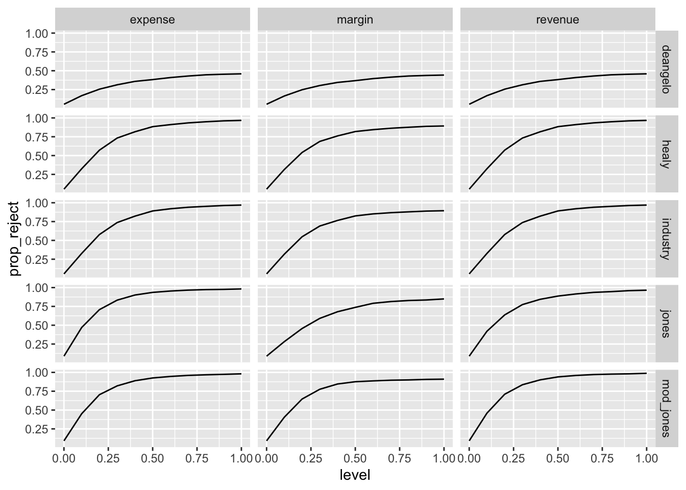
16.3.1 Discussion questions
How do the results in Figure 16.1 compare with those in Figure 4 of Dechow et al. (1995)?
According to the SEC’s filing referenced above related to B&L, “B&L recognized, in contravention of GAAP and the Company’s own revenue recognition policies, $42.1 million of revenue, resulting in at least a $17.6 million, or 11%, overstatement of the net income originally reported for its 1993 fiscal year.” According to a subsequent SEC filing, B&L’s total assets for 1994 were $2,457,731,000 (it seems reasonable to assume that the 1993 value was not radically different from this). Based on this information (plus any information in the SEC’s filing), which of Dechow et al. (1995)’s three categories did B&L’s earnings management fall into? What is the approximate magnitude relative to the \(x\)-axes of the plots in Figure 4 of Dechow et al. (1995) (or the equivalent above)? Based on these data points, what is the approximate estimated probability of the various models detecting earnings management of this magnitude?
What do you view as the implications of the power analysis conducted above for research on earnings management? Are these implications consistent with the extensive literature on earnings management subsequent to Dechow et al. (1995)? If so, explain why. If not, how would you reconcile the inconsistencies?
Does each of the three forms of earnings management implemented in
manipulate()above agree precisely with the corresponding description in Dechow et al. (1995, pp. 201–202)? If not, does one approach seem more correct than the other? (Note that one issue arises with negative or zero net income ratio. How are such cases handled by Dechow et al. (1995) and bymanipulate()?)
See https://en.wiktionary.org/wiki/operationalizable#English.↩︎
As in Chapter 15, we supplement data on
comp.fundawith SIC codes fromcomp.company.↩︎Because we need lagged values for most analyses, in only collecting data from 1950, we will lose that first year from most analyses. It is unclear whether Dechow et al. (1995) collected data for 1949 to be able to use 1950 firm-years in their analysis, but it is unlikely to have much of an impact (there are few firms in the data for 1950) and it would be easy to tweak if we wanted to include 1950 in our analysis.↩︎
Our sampling approach deviates from that in Dechow et al. (1995), where firm-years are selected (without replacement) subject to the constraint that “a firm-year is not selected if its inclusion in the random sample leaves less than ten unselected observations for the estimation period.” One important difference is that the approach in Dechow et al. (1995) could lead to a firm having two years of earnings management. There seems to be little upside in this, while our approach is much simpler to code and unlikely to impact results in a significant way.↩︎
We put
fit_jones()andfit_mod_jones()outside the function for reasons that will become clear if you attempt the exercises.↩︎Chapter 19 of Wickham (2019) has more details on this “unquote” operator
!!.↩︎We explore the meaning of “differently” in the discussion questions.↩︎