20 Instrumental variables
Angrist and Pischke (2008, p. 114) describe instrumental variables (IVs) as “the most powerful weapon in the arsenal” of empirical researchers. Accounting researchers have long used instrumental variables in an effort to address concerns about endogeneity (Larcker and Rusticus, 2010; Lennox et al., 2012) and continue to do so.
Unfortunately, faulty reasoning about instruments is common in accounting research. Larcker and Rusticus (2010) lament that “some researchers consider the choice of instrumental variables to be a purely statistical exercise with little real economic foundation” and call for “accounting researchers … to be much more rigorous in selecting and justifying their instrumental variables.” And a review of instrumental variable applications conducted by Gow et al. (2016) suggests that accounting researchers have paid little heed to the suggestions and warnings of Larcker and Rusticus (2010), Lennox et al. (2012), and Roberts and Whited (2013).
As we shall demonstrate in this chapter, the requirements for valid instruments are demanding and the supply of plausibly valid IVs in accounting research to date is arguably zero. As such, the use of IV should be rare, and readers, editors, and reviewers should sceptically apply the requirements discussed below to any proposed IV.
The code in this chapter uses the packages listed below. For instructions on how to set up your computer to use the code found in this book, see Section 1.2. Quarto templates for the exercises below are available on GitHub.
20.1 The canonical causal diagram
Gow et al. (2016) argue that evaluating instrumental variables requires careful theoretical causal, rather than statistical, reasoning. Statistical reasoning is what you will find in most econometrics textbooks, which discuss requirements regarding probability limits (e.g., \(\mathrm{plim}\;Z^{\mathsf{T}}X \neq 0\) and \(\mathrm{plim} \;Z^{\mathsf{T}}\epsilon = 0\)). In practice, you are more likely to see researchers invoking ideas such as the “only through” criterion, which are better understood as causal ideas.
Causal diagrams provide a useful framework for highlighting the requirements for a valid instrument and thus (hopefully) avoiding incorrect reasoning. The causal diagram in Figure 20.1 can be viewed as the “canonical” causal diagram for instrumental variables.
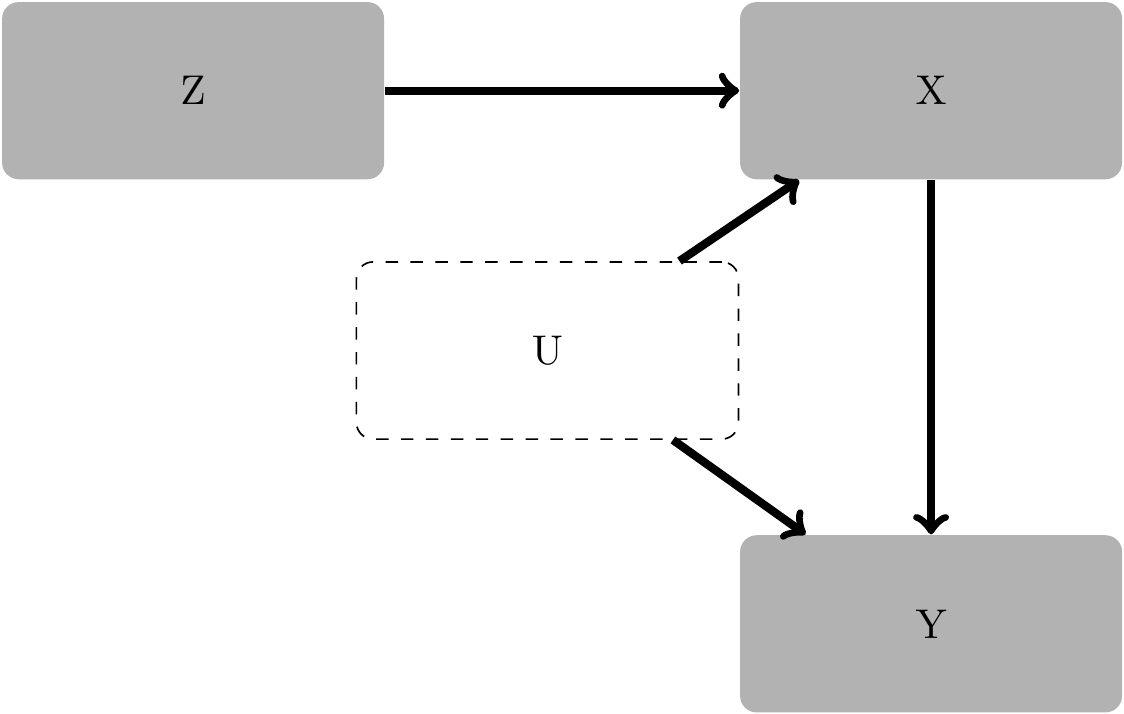
Figure 20.1 is similar to the “\(Z\) is a confounder” figure we saw in Chapter 4, but for two differences. First, the confounding variable \(U\) is not observed. (What was labelled \(Z\) in Section 4.2 is now labelled \(U\) because of the convention of using \(Z\) for instrumental variables, which we follow here.) Our reasoning in Chapter 4 suggested that if we don’t condition on \(U\), the coefficients obtained from a regression of \(Y\) on \(X\) will be biased estimates of the causal effect of \(Y\) on \(X\). But with \(U\) unobserved, we simply cannot use a strategy of conditioning on \(U\) to produce valid causal inferences.
The second difference is that we have a new variable \(Z\), which is our instrumental variable. It turns out that a variable with the attributes that \(Z\) has in the causal diagram will (subject to certain additional technical requirements) allow us to get consistent estimates of the causal effect of \(X\) on \(Y\).
Figure 20.1 implies three critical features of \(Z\). First, \(Z\) is random. This is implied by the absence of any arrows into \(Z\). Second, \(Z\) has a causal effect on \(X\), which is indicated by the arrow from \(Z\) to \(X\). (Later we will see that the strength of the causal relation between \(Z\) and \(X\) is important for reliable inferences.) Third, there is no direct causal effect of \(Z\) on any variable other than \(X\). This is the “only through” criterion we mentioned earlier: the effect (if any) of \(Z\) on \(Y\) goes “only through” \(X\).
Consistent with the causal perspective we take here, Angrist and Pischke (2008, p. 117) argue that “good instruments come from a combination of institutional knowledge and ideas about the process determining the variable of interest.” For example, Angrist (1990) studied a draft lottery used to determinate eligibility for being drafted into military service to estimate effects of such service on long-term labour market outcomes. In the setting of Angrist (1990), it was well that the lottery was random and the mapping from the lottery to draft eligibility was well understood. Furthermore, there are good reasons to believe that the draft lottery did not affect anything directly except for draft eligibility.1
It is perhaps worth reiterating that arguing that the only effect of an instrument on the outcome variable of interest is via the treatment of interest does not suffice to establish a valid instrument. Even if the claim that \(Z\) only affects \(Y\) via its effect on \(X\) is true, the researcher also needs to argue that variation in the instrument (\(Z\)) is as-if random. For example, if \(Z\) is a function of a variable \(W\) that is also associated with \(Y\), then even if the “only through” criterion is satisfied (i.e., the only effect of \(Z\) on \(Y\) occurs via \(X\)), IV estimates of the effect of \(X\) on \(Y\) will in general be biased.2
Unfortunately, there are few (if any) accounting variables that meet the requirement that they randomly assign observations to treatments and do not affect the outcome of interest outside of effects on the treatment variable. Sometimes researchers turn to lagged values of endogenous variables or industry averages as instruments, but these too are problematic.3
20.2 Estimation
We now examine the estimation of IV in detail. Suppose that the outcome variable is generated by the following equation:
\[y = X \beta + \epsilon\]
where \(X\) is an \(n \times k\) matrix and \(\beta\) is a \(k\)-element vector of coefficients.
The goal of a researcher is to estimate \(\beta\), which provides the causal effect of \(X\) on \(y\). The OLS estimator is \[ \widehat{\beta}_\mathrm{OLS} = (X^{\mathsf{T}} X)^{-1} X^{\mathsf{T}} y = (X^{\mathsf{T}} X)^{-1} X^{\mathsf{T}} (X \beta + \epsilon) = \beta + (X^{\mathsf{T}} X)^{-1} X^{\mathsf{T}} \epsilon\]
When \(X\) and the other unmeasured, causal variables collapsed into the \(\epsilon\) term are correlated, the OLS estimator is generally biased and inconsistent for \(\beta\).
Note that the predicted values from an OLS regression are calculated as \[ \widehat{y} =X \widehat{\beta}_\mathrm{OLS} = X (X^{\mathsf{T}} X)^{-1} X^{\mathsf{T}} y = P_X y\] Where \(P_X\) is defined as \[ P_X =X(X^{\mathsf{T}} X)^{-1}X^{\mathsf{T}}\] Thus we can express the predicted values as \[ \widehat{y} = X \widehat{\beta} = P_X y\] Here \(P_X\) is an example of a projection matrix.4 For a matrix \(W\) and a vector \(v\), the multiple of the projection matrix \(P_W\) and \(v\) projects \(v\) into the linear subspace defined by \(W\). If \(W\) is an \(n \times k\) matrix, then \(P_W\) will be an \(n \times n\) matrix that is symmetric (meaning that \(P_X^{\mathsf{T}} = P_X\)) and idempotent (meaning that \(P_W \times P_W = P_W\)).5
Suppose we have a set of \(r\) variables \(Z\) comprising both exogenous elements of \(X\) and instrumental variables where \(r \geq k\).
Definition 20.1 (Convergence in probability) A sequence of random variables \(\{x_n: n = 1, 2, \dots \}\) converges in probability to a constant \(a\) if for all \(\epsilon > 0\), \[ \mathbb{P}\left( \left| x_n - a \right| > \epsilon \right) \to 0 \text{ as } n \to \infty\] In such a case, we say that \(a\) is the probability limit (or plim) of \(x_n\) and write \(\operatorname{plim} x_n = a\).
Definition 20.2 (Consistency) Given a model \(y = X \beta + \epsilon\), an estimator \(\hat{\beta}\) is consistent for \(\beta\) if \[ \operatorname{plim} \hat{\beta} = \beta \]
Asymptotic properties of estimators are often sufficiently mathematically tractable that we can often demonstrate that estimators have desirable properties—such as consistency—even when it is difficult to evaluate their finite-sample properties. The conceptual leap we make as applied researchers is that an estimator with desired asymptotic properties will perform well in real-world samples that are sufficiently large, albeit finite.
We can use \(Z\) to calculate the two-stage least squares (2SLS) estimator as \[ \widehat{\beta}_\mathrm{2SLS} = (X^{\mathsf{T}} P_Z X)^{-1}X^{\mathsf{T}} P_Z y,\] Denoting \(\hat{X}\) as \(P_Z X\), we could regress \(y\) on \(\widehat{X}\) using OLS to get the 2SLS estimator. \[ \begin{aligned} \hat{\beta} &= (\hat{X}^{\mathsf{T}} \hat{X})^{-1} \hat{X}^{\mathsf{T}} y \\ &= \left((P_Z X)^{\mathsf{T}}P_Z X \right)^{-1} (P_Z X)^{\mathsf{T}} y \\ &= \left(X^{\mathsf{T}} P_Z^{\mathsf{T}} P_Z X \right)^{-1} (P_Z X)^{\mathsf{T}} y \\ &= \left(X^{\mathsf{T}} P_Z X \right)^{-1} X^{\mathsf{T}} P_Z y \\ \end{aligned} \] (Note that we used the idempotency and symmetry of \(P_Z\) in this analysis.)
We can rewrite the underlying model as \[ y = \hat{X} \beta + (X - \hat{X}) \beta + \epsilon \] We can think of \(\widehat{\beta}_\mathrm{2SLS}\) as the estimator from this model (i.e., from regressing \(y\) on \(\widehat{X}\)) with an error term equal to \((X - \hat{X}) \beta + \epsilon\).
Here \(\hat{X}\) and \((X - \hat{X})\) are, respectively, the fitted values and residuals from an OLS regression of \(X\) on \(Z\), so \(\hat{X}^{\mathsf{T}} (X - \hat{X}) = 0\) and \(\operatorname{plim} N^{-1} \hat{X}^{\mathsf{T}} (X - \hat{X}) \beta = 0\).
Given that \[ N^{-1} \hat{X}^{\mathsf{T}} \epsilon = N^{-1} X^{\mathsf{T}} P_{Z} \epsilon = N^{-1} X^{\mathsf{T}} Z (N^{-1} Z^{\mathsf{T}} Z)^{-1} N^{-1} Z^{\mathsf{T}} \epsilon \]
we have \(\operatorname{plim} N^{-1} \hat{X}^{\mathsf{T}} \epsilon = 0\) so long as \(\operatorname{plim} N^{-1} Z^{\mathsf{T}} \epsilon = 0\), which is implied by Figure 20.1. This shows that \(\widehat{\beta}_\mathrm{2SLS}\) is a consistent estimator for \(\beta\). This result depends on the linearity of the model and does not generalize to non-linear models.6
A careful reader might note that we have not used the causal diagram from the previous subsection in this analysis. A heuristic analysis of the 2SLS estimator given the canonical causal diagram can be found in Cunningham (2021, pp. 323–329).
20.3 Reasoning about instruments
Larcker and Rusticus (2010, p. 189) find that in a typical accounting research paper, “there is almost no discussion regarding the choice of specific variables for instruments (only slightly more than half of the papers discuss the instruments at all). Researchers do not rigorously discuss why the variables selected as instruments are assumed to be exogenous … nearly 80% of the papers provide no justification for the choice of instrument whatsoever.”
But, even when researchers do attempt to evaluate instruments, confusion and loose reasoning seem common. For example, in the rare cases where instruments are justified, many appear to focus on what Roberts and Whited (2013, p. 514) describe as “the question one should always ask of a potential instrument [namely] does the instrument affect the outcome only via its effect on the endogenous regressor?” But a focus on this question cannot come at the expense of discussion of the requirement that the instrument be (as-if) random.
The discussion of instrument validity of Roberts and Whited (2013, p. 514) actually provides a good case study for accounting researchers, as they are writing to enhance reasoning about endogeneity in finance, a field closely related to accounting research.
The setting explored by Roberts and Whited (2013) is that of Bennedsen et al. (2007), who “find that family successions have a large negative causal impact on firm performance” [p. 647]. While Roberts and Whited (2013) proceed with fairly loose verbal reasoning, we think it is helpful to recapitulate their analysis using a series of questions implied by the requirements for a valid instrument.
One baseline requirement for this analysis is that we need to have a clear idea of what the instrument is, what the treatment variable is, and what the outcome is.
The quoted sentence from Bennedsen et al. (2007) identifies the treatment (family succession) and the outcome of interest (firm performance). The instrument used by Bennedsen et al. (2007) is the gender of the first-born child of a departing CEO.
A second critical element of this analysis is that we use causal reasoning rather than statistical reasoning. While an underlying causal model will imply statistical relations, it is problematic to substitute statistical analysis of observed data for such causal reasoning.
Here are the questions:
Is the instrument (as-if) random? The question is addressed quite directly by Bennedsen et al. (2007). Our knowledge of human biology tells us that the sex of a child is essentially random at time of conception. And, as “over 80 percent of first-child births [in the sample] occurred prior to 1980, before current techniques to identify the gender of children were widespread”, there is little reason to doubt that the sex of live births isn’t similarly random.
-
Does the instrument have a direct causal effect on the treatment variable? Here Bennedsen et al. (2007) rely on statistical evidence: “We show that the gender of the first-born child of a departing CEO is strongly correlated with the decision to appoint a family CEO: The frequency of family transitions is 29.4% when the first-born child is female and increases to 39% (a 32.7% increase) when the first-born is male.” But it is important that this link be causal. A merely statistical association between \(Z\) and \(X\) is problematic if we do not have a clear causal explanation. If \(X\) and \(Z\) are associated for unexplained reasons, it is difficult to rule out the possibility that those unexplained reasons include variables that drive both \(X\) and \(Z\) or effects of \(Z\) on variables other than \(X\) that might be associated with \(Y\). Either of these alternatives would undermine the validity of \(Z\) as an instrument and thus need to be ruled out.
What Bennedsen et al. (2007) appear to need here is that, for a proportion of the firms in the sample, family succession is caused by the first-born child being a son rather than a daughter. The paper mentions “primogeniture” a couple of times and perhaps we can assume that this mechanism exists based on general knowledge of Danish customs, but more discussion beyond the statistics might have been helpful for readers with little knowledge of Danish family dynamics beyond what is depicted in Hamlet.
-
Does the instrument affect the outcome only through its effect on the treatment variable? Again Bennedsen et al. (2007) rely on statistical evidence: “We find that firms’ profitability, age, and size do not differ statistically as a function of the gender of the first child. Moreover, the family characteristics of departing CEOs are comparable.” But it is not possible to test the “only through” assumption statistically, instead we need “compelling arguments relying on economic theory and a deep understanding of the relevant institutional details” (Roberts and Whited, 2013, p. 515).
In this regard, the requirements are steep and Bennedsen et al. (2007) arguably fall short. One reason to doubt the “only through” requirement is the sheer amount of time between assignment of the instrument and the assignment of treatment (family succession) and the presumed preference for first-born sons to take over. There might be 40 or 50 or more years between the birth of the first child and CEO succession. The “only through” requirements means that the sex of the first child does not affect anything about the firm other than family succession. This means that nothing about the management of the firm prior to CEO succession is affected by the increased likelihood that the firm will continue to be managed by the family after the CEO leaves. This rules out management assignment decisions that are intended to groom a family member for a CEO role, as these could affect performance through channels other than the mere fact of family succession. It also rules out decisions about the structure or performance of the firm (e.g., which portions of the firm are retained and how much effort is exerted in running it) prior to succession.
In summary, Roberts and Whited (2013) explicitly identify only Question 3 as the critical one, but in a setting where it is Questions 1 and 2 that appear to have the correct answer. But focusing on Question 3 and ignoring Question 1 can be problematic in practice, as we shall see in the next subsection.
An important caveat to the somewhat negative evaluation of the reasoning in Bennedsen et al. (2007) is that just because there are holes in the arguments for an instrument’s validity does not mean that one cannot make causal inferences. It just means that the causal reasoning has to be more circumspect and rule out alternative causal pathways from the (plausibly random) instrument to the outcome.
20.4 “Bullet-proof” instruments
While some accounting researchers appear to believe that statistical tests can be used to evaluate whether an instrument is “valid” (see Larcker and Rusticus, 2010), there are no simple statistical tests for the validity of instruments. Indeed, many studies choose to test the validity of their instrumental variables using statistical tests, but such tests of instruments are of little value in practice.
In this section, we examine what we might “achieve” if we relax the requirement for an instrument to be random (i.e., we skip Question 1 above) and rely on statistical tests to address the concerns raised by this hypothetical reviewer.7
Suppose that we have \(y = X \beta + \epsilon\), with \(\rho(X, \epsilon) = 0.2\) and \(\beta = 0\). This means that there is no causal relation between \(X\) and \(y\), but we have an endogeneity issue and thus might despair our inability to get good inferences about the causal relation between \(X\) and \(y\).
Below we create a function—generate_data()—to generate data with the properties and parameter values discussed above, then run it to produce df. Here we have \(X\) and \(\epsilon\) that are bivariate-normally distributed with mean \(0\) and variance \(1\).
We know that OLS regression estimates using these data will be biased and therefore will not support credible causal inferences.
But, wait. We have a “solution”! We can simply create three instruments: \(z_1 = x + \eta_1\), \(z_2 = \eta_2\), and \(z_3 = \eta_3\), where \(\sigma_{\eta_1} = \sigma_{\eta_2} = \sigma_{\eta_3} \sim N(0, 0.09)\) and independent. We can even make an R function generate_ivs() to do this:
We apply generate_ivs() to our data setdf` to create a data set with generated instruments.
df_ivs <- generate_ivs(df)Now, do these instruments pass the “only through” requirement? Clearly there is no relation between any of the instruments and any other variable except for \(z_1\), which is only associated with other variables through its relation with \(X\). So, “yes”!
What happens when we estimate IV using these instruments? We run an OLS regression and an IV regression using our generated instruments.
The results of these regressions are shown in Table 20.1.
modelsummary(fms,
             estimate = "{estimate}{stars}",
             coef_rename = c('fit_X' = 'X'),
             gof_map = c("nobs", "r.squared"),
stars = c('*' = .1, '**' = 0.05, '***' = .01))| OLS | IV | |
|---|---|---|
| (Intercept) | -0.054* | -0.055* |
| (0.031) | (0.031) | |
| X | 0.184*** | 0.174*** |
| (0.031) | (0.032) | |
| Num.Obs. | 1000 | 1000 |
| R2 | 0.035 | 0.035 |
There we see that our IV regressions deliver statistically significant positive coefficient on \(X\) and, given our use of IV, we might feel comfortable attaching a causal interpretation to this coefficient. (Of course, we know in this scenario that the true \(\beta\) is zero; in practice, we would not know this.)
Of course, a sceptical reviewer might ask us to justify our generated instruments beyond the “only through” argument we made above. For example, it is common to ask whether our instruments pass a test of overidentifying restrictions. Such tests apply when we have more instruments than endogenous variables for which we need instruments and typically posit that at least one instrument is valid and ask whether we can reject the null hypothesis that the other instruments are valid.
The sceptical reviewer might also ask us to provide evidence that we do not have weak instruments.8 Weak instruments lead to bias in small samples (Stock et al., 2002).
We can extract statistics related to standard tests as follows:
iv <- fms[["IV"]]
iv_sargan <- iv$iv_sargan
Sargan.stat <- iv_sargan$stat
Sargan.p <- iv_sargan$p
ivf1 <- fitstat(iv, "ivf1", simplify = TRUE)
F.stat <- ivf1$stat
F.p <- ivf1$p
Here we have a Sargan test statistic of 1.32 (p-value of 0.52). So we “pass” the test of overidentifying restrictions. Based on a test statistic of 30, which easily exceeds the thresholds suggested by Stock et al. (2002), the null hypothesis of weak instruments is rejected as we have an \(F\)-stat of 3773. So we can report to our sceptical reviewer that our instruments are “good”. And we have “results”. Yay!
But maybe we got lucky. To test this, we create a function run_simulation() that we can use to see if this pattern is robust.
run_simulation <- function(run) {

  iv <-
    generate_data() |>
    generate_ivs() |>
    feols(y ~ 1 | X ~ z_1 + z_2 + z_3, data = _)

  iv_sargan <- iv$iv_sargan
  ivf1 <- fitstat(iv, "ivf1", simplify = TRUE)

  return(
    tibble(
      run = run,
      coeff = iv$coeftable["fit_X", "Estimate"],
      p.value = iv$coeftable["fit_X", "Pr(>|t|)"],
      Sargan.stat = iv_sargan$stat,
      Sargan.p = iv_sargan$p,
      F.stat = ivf1$stat,
      F.p = ivf1$p))
}
The following code runs 1000 simulations and extracts some test statistics.
The results of our simulation analysis are as follows:
- The mean estimated coefficient on \(X\) is 0.2, which is statistically significant at the 5% level 100% of the time. Note that this coefficient is close to \(\rho(X, \epsilon) = 0.2\) , which is to be expected given how our data were generated.
- The null hypothesis of weak instruments is rejected 100% of the time using a test statistic of 30, which easily exceeds the thresholds suggested by Stock et al. (2002).
- The test of overidentifying restrictions fails to reject a null hypothesis of valid instruments (at the 5% level) 92.9% of the time.
Again, hooray! Our hypothetical referee should be satisfied almost always. But we know that these results are bogus. The problem: the instrument \(Z\) is not random; it’s a function of \(X\) and essentially just as endogenous as \(X\) is.
While the generated instruments we used above might seem a bit fanciful, they are probably not very different from instruments such as lagged values or industry averages (\(z_1\)) or random items plucked from Compustat (more like \(z_2\) or \(z_3\)), which are not unheard of in actual research.
This example shows that completely spurious instruments can easily pass tests for weak instruments and tests of overidentifying restrictions and yet deliver bad inferences.
20.5 Causal diagrams: An application
To illustrate the application of causal diagrams to the evaluation of instrumental variables, we consider Armstrong et al. (2013). Armstrong et al. (2013) study the effect of shareholder voting (\(\textit{Shareholder support}_{t}\)) on future executive compensation (\(\textit{Comp}_{t+1}\)). Because of the plausible existence of unobserved confounding variables that affect both future compensation and shareholder support, a simple regression of \(\textit{Comp}_{t+1}\) on \(\textit{Shareholder support}_{t}\) and controls would not allow Armstrong et al. (2013) to obtain an unbiased or consistent estimate of the causal relation.
Among other analyses, Armstrong et al. (2013) use an instrumental variable to estimate the causal relation of interest. Armstrong et al. (2013) claim that their instrument is valid. Their reasoning is represented graphically in Figure 20.2. By conditioning on \(\textit{Comp}_{t-1}\) and using Institutional Shareholder Services (ISS) recommendations as an instrument, Armstrong et al. (2013) argue that they can identify a consistent estimate of the causal effect of shareholder voting on \(\textit{Comp}_{t+1}\), even though there is an unobserved confounder, namely determinants of future compensation observed by shareholders, but not the researcher.9
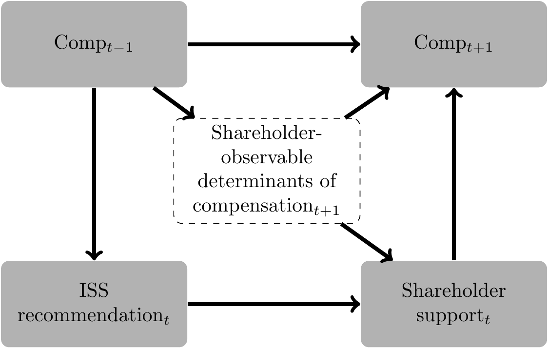
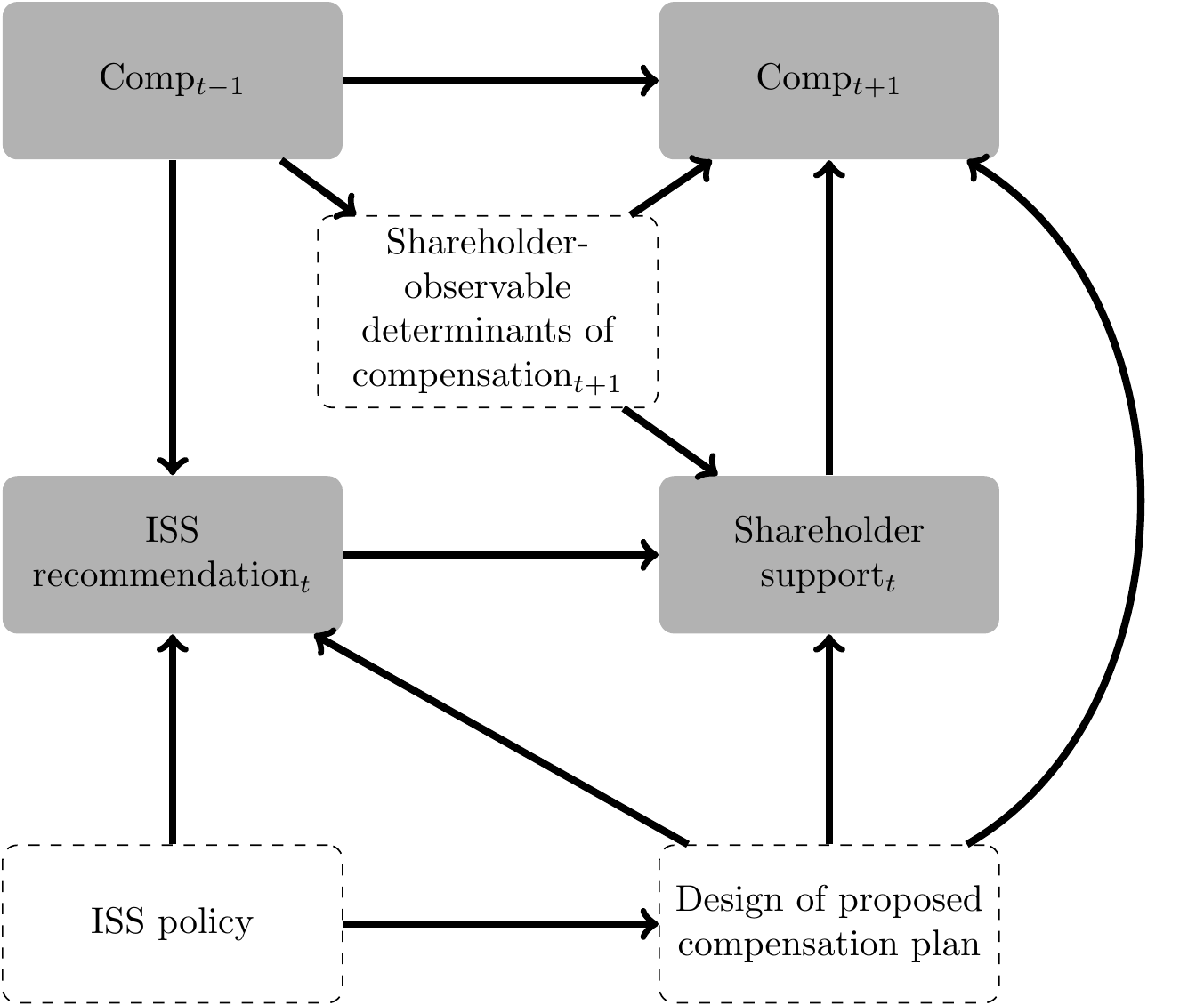
While the authors note this possibility: “validity of this instrument depends on ISS recommendations not having an influence on future compensation decisions conditional on shareholder support (i.e., firms listen to their shareholders, with ISS having only an indirect impact on corporate policies through its influence on shareholders’ voting decisions)”, they are unable to test the assumption (Armstrong et al., 2013, p. 912). Unfortunately, this assumption seems inconsistent with the findings of Gow et al. (2013), who provide evidence that firms calibrate compensation plans (i.e., factors that directly affect \(\textit{Comp}_{t+1}\)) to comply with ISS’s policies so as to get a favourable recommendation from ISS. As depicted in Figure 20.3, this implies a back-door path from \(\textit{Comp}_{t+1}\) into \(\textit{ISS recommendation}_t\), suggesting that the instrument of Armstrong et al. (2013) is not valid.10
The careful reader will note that we did not need to address the randomness of the instrument (i.e., “Question 1” from above) to conclude that the instrument is problematic. It is implicitly assumed in the first causal diagram that \(\textit{ISS recommendation}_t\) is random conditional on \(\textit{Comp}_{t-1}\), which would need to be included in the regression even based on the first causal diagram. A fuller analysis of the first causal diagram is beyond the scope of the current version of this course, as it would require results not covered herein.
20.6 Further reading
Given the difficulty of identifying credible instruments in accounting research, we have eschewed the replication of actual papers in this chapter. The challenges with IVs seem more apparent with idealized settings provided by simulation analysis. We direct readers interested in textbook treatments of IVs at a similar or slightly more advanced level to Cunningham (2021) and Adams (2020), each of which provides an up-to-date treatment of issues related to IV estimation. Chapter 4 of Angrist and Pischke (2008) provides a good introduction to IVs with several examples. More on instrumental variables and causal diagrams can be found in Chapter 7 of Pearl (2009).
20.7 Discussion questions and exercises
In the 1960s and early 1970s, American men were at risk of being drafted for military service. Each year from 1970 to 1972, draft eligibility was prioritized based on the results of a lottery over birthdays. A random number was assigned to the birthdays of 19-year-olds. Those whose birthday was associated with a random number below the cut-off were draft-eligible; the other 19-year-olds were not draft-eligible. Angrist and Pischke (2008) point out that, “in practice, many draft-eligible men were still exempted from service for health or other reasons, while many men who were draft-exempt nevertheless volunteered for service.” Using an indicator for draft lottery number being below the cut-off as an instrumental variable, Angrist (1990) finds that those who served in Vietnam earned significantly less than their peers even in 1981. Try to draw the causal diagram for this analysis and apply the three questions outlined above to this setting. What assumptions are needed for the answer to each question to be “yes”? How might these assumptions be violated?
Ahern and Dittmar (2012) study a rule requiring firms in Norway to appoint female directors and “use the pre-quota cross-sectional variation in female board representation to instrument for exogenous changes to corporate boards following the quota.” What is the significance of the discussion suggesting that “the quota was implemented without the consent of business leaders” (2012, p. 145)? What about the discussion (2012, p. 155) suggesting that the rule was not anticipated?
You and a co-author are interested in studying the effect of independent directors on financial reporting quality. You conjecture that independent directors demand better financial reporting, as they are less likely to benefit from obfuscation of performance than non-independent directors, who are often employees of the firm. However, you are concerned that causation may run in the opposite direction; firms with better financial reporting quality may have more independent directors on their boards. Provide some arguments for the existence of reverse causation. How persuasive do you find these arguments?
-
In response to a request by the SEC in February 2002, the major US exchanges (NYSE and Nasdaq) proposed changes to listing standards that would require firms to have a majority of independent directors. In 2003, the SEC approved these changes and required that firms comply by the earlier of (i) the first annual shareholder meeting after January 15, 2004 and (ii) October 31, 2004. Your co-author argues that this change was “exogenous”, as it was not driven by the decisions of individual firms, and this fact allows you to estimate a causal effect.
Does “exogeneity” as used by your co-author mean the same thing as exogeneity for the purposes of econometric analysis? Does the former notion imply the latter? Think of “examples” to support your arguments (an example could be a simple model, a numerical argument, or a verbal description of a real or imagined scenario).
More specifically, your co-author argues that the change in the number of independent directors imposed on the firm by the new rules is exogenous and thus could be used as an instrument for your study. Armstrong et al. (2014) examine the changes in listing standards above and use “the minimum required percentage change in independent directors,
Min % change ID, as an instrument” in studying the effect of independent directors on firm transparency. What are the parallels between the setting of Armstrong et al. (2014) and that of Ahern and Dittmar (2016)? Do the two papers use the same basic approach, or are there important differences between their approaches? The objective of Cohen et al. (2013) “is to investigate how governance regulations in SOX and the exchanges are associated with chief executive officers’ incentives and risk-taking behavior.” What is the treatment of interest in Cohen et al. (2013)? What are the outcomes of interest? Cohen et al. (2013) state that “our dependent variables, namely, investment and executive incentive compensation, are likely to be determined jointly. As such, the parameter estimates from ordinary least squares (OLS) are likely to be biased. Our empirical analyses address the issue by using simultaneous equations models.” What “exclusion restrictions” are implied by Panel A of Table 4? What does the implied causal diagram look like? How persuasive do you find the approach of Cohen et al. (2013) to be?
# Set parameters
n <- 10000; max_d <- 10
set.seed(1); z <- rlnorm(n)
a <- 1
gamma <- 3; b <- gamma * z
alpha <- 100; beta <- 10; sd_epsilon <- 5

d_opt_fun <- function(a, b, min_d = 0) {

  v <- function(x) -a * x^2 + b * x

  opts <- min_d:max_d
  vals <- sapply(opts, v)
  d_opt <- opts[vals == max(vals)]
  d_opt
}

d_opt_fun <- Vectorize(d_opt_fun)

# Calculate firm value, etc., at t = 0
df <-
  tibble(a, b) |>
  mutate(epsilon_0 = rnorm(n, sd = sd_epsilon),
         V_0 = alpha + beta * b + epsilon_0,
         d_0 = d_opt_fun(a, b))

# Add firm value, etc., at t = 1
min_d <- 3
df_1 <-
  df |>
  mutate(epsilon_1 = rnorm(n, sd = sd_epsilon),
         V_1 = alpha + beta * b + epsilon_1,
d_1 = d_opt_fun(a, b, min_d = min_d))-
Suppose the existence of a world of Sneetches.11 There are two kinds of Sneetches:
Now, the Star-Belly Sneetches
Had bellies with stars.
The Plain-Belly Sneetches
Had none upon thars.
—Dr. SeussIn the Sneetch world, there are 10,000 (
n) firms, each with a board of 10 (max_d) directors. The number of Plain-Belly directors \(d_i\) is set by firm \(i\) as \[d_i = {\underset {x\in [\underline{d}, \overline{d}]}{\operatorname {arg\,max} }}\, v_i(x) = -a_i x^2 + b_i x \] where \(a_i = 1\) and \(b = \gamma z_i\), \(\gamma = 3\) and \(z_i\) is log-normally distributed with default parameters of \(\mu=0\) and \(\sigma=1\). We start with \(\underline{d} = 0\) and \(\overline{d} = 10\). The remaining \(10 - d_i\) directors would be Star-Belly Sneetches.The value of firm \(i\) at time \(t=0\) is given by the equation: \[ V_{i0} = \alpha + \beta \times b_i + \epsilon_0 \] where \(\alpha = 100\), \(\beta = 10\) and \(\epsilon \sim N(0, \sigma_{\epsilon})\), where \(\sigma_{\epsilon} = 5\). The Sneetches then pass new legislation requiring every board to have at least three Plain-Belly directors at time \(t=1\). The value of firm \(i\) at time \(t=1\) is given by the equation: \[ V_{i1} = \alpha + \beta \times b_i + \epsilon_{i1} \] The code in Listing 20.1 starts by setting the parameters discussed above and generating \(\gamma_i\) (
gamma). The code then generates the value of each of the 10,000 firms at time \(t=0\) (V_0), as well as the number of Plain-Belly directors chosen by each firm at \(t=0\) to maximize \(v_i(\cdot)\) (d_0). These values are stored indf.The code in Listing 20.1 then sets
min_dto reflect the requirement of the legislation coming into force for \(t = 1\). The code then generates the value of each firm at \(t=1\) (V_1) and the number of Plain-Belly directors chosen by each firm at \(t=1\) (d_1), which involves maximization of \(v_i(\cdot)\) subject to the new constraint that \(d_i \geq 3\). We assume that neither \(a_i\) nor \(b_i\) is observable to the researcher.Expressed in terms of \(a_i\) and \(b_i\), what value of \(x\) maximizes \(v_i(x)\) when there is no constraint (as is true at \(t = 0\))?
What issue do we have in using this maximum to select the number of Plain-Belly directors on a board?
What does
d_opt_fun()in Listing 20.1 do to handle this issue?What does the function
Vectorize()do in Listing 20.1? (Hint: Use? Vectorizein R to learn more about this function.)Using OLS and data in
df_1after running the code in Listing 20.1, estimate the relationship between firm value at time \(t=1\) (\(V_1\)) and the number of Plain-Belly directors on the board (\(d_1\)).Using the data in
df_1, estimate an IV regression using the strategy of Ahern and Dittmar (2012).Using the data in
df_1, estimate an IV regression using the strategy of Armstrong et al. (2014) (note that rather thanMin % change X, you might use something likeMin change X, as the denominator is 10 for all observations). Hint: Thepmin()function in R gives the point-wise minimum of two vectors of values (e.g.,pmin(x, y)will return the lower ofxandyfor each pair.)What is the true causal effect of Plain-Belly directors on firm value? Do the strategies of either Ahern and Dittmar (2012) or Armstrong et al. (2014) correctly estimate this effect?
Though some have questioned the exclusion restriction even in this case, arguing that the outcome of the draft lottery may have caused some, for example, to move to Canada (see Imbens and Rubin, 2015).↩︎
In the case of Angrist (1990), the requirement that \(Z\) be random was plausibly satisfied by the use of a lottery.↩︎
See Reiss and Wolak (2007) for a discussion regarding the implausibility of general claims that industry averages are valid instruments.↩︎
See Appendix A for more on projection matrices.↩︎
See Appendix A for more on symmetric and idempotent matrices.↩︎
The material in this subsection is based on material on p.189 of Cameron and Trivedi (2005).↩︎
Much of this section is based on an example that first appeared in Gow et al. (2016).↩︎
See suggestions regarding further reading at the end of the chapter for more about these tests.↩︎
In Figure 20.2, we depict the unobservability of this variable (to the researcher) by putting it in a dashed box. Note that we have omitted the controls included by Armstrong et al. (2013) for simplicity, though a good causal analysis would consider these carefully.↩︎
Armstrong et al. (2013) recognize the possibility that the instrument they use is not valid and conduct sensitivity analysis to examine the robustness of their result to violation of the exclusion restriction assumptions. This analysis suggests that their estimate is highly sensitive to violation of this assumption.↩︎
The interested reader can learn more about Sneetches in Dr Seuss’s The Sneetches and Other Stories, available on (for example) Amazon: https://www.amazon.com/dp/0394800893.↩︎