19 Natural experiments revisited
In this chapter, we return to the topic of natural experiments. We first discuss the notion of registered reports, their purpose, and their limitations. We then focus on an experiment (“Reg SHO”) run by the US Securities and Exchange Commission (SEC) and studies that examined the effects of Reg SHO, with a particular focus on one study (Fang et al., 2016) that exploited this regulation to study effects on earnings management.
This chapter provides opportunities to sharpen our skills and knowledge in a number of areas. First, we will revisit the topic of earnings management and learn about some developments in its measurement since Dechow et al. (1995), which we covered in Chapter 16. Second, we further develop our skills in evaluating claimed natural experiments, using Reg SHO and the much-studied setting of broker-closure shocks. Third, we explore the popular difference-in-differences approach, both when predicated on random assignment and when based on the so-called parallel trends assumption in the absence of random assignment. Fourth, we will have an additional opportunity to apply ideas related to causal diagrams and causal mechanisms (covered in Chapters 4 and 18, respectively). Fifth, we will revisit the topic of statistical inference, using this chapter as an opportunity to consider randomization inference. Sixth, we build on the Frisch-Waugh-Lovell theorem to consider issues associated with the use of two-step regressions, which are common in many areas of accounting research.
The code in this chapter uses the packages listed below. We load tidyverse because we use several packages from the Tidyverse. For instructions on how to set up your computer to use the code found in this book, see Section 1.2. Quarto templates for the exercises below are available on GitHub.
This chapter is longer than others in the book, so we have made it easier to run code from one section without having to run all the code preceding it. Beyond that, the code in each of Sections 19.1–19.3 and 19.5 is independent of code in other parts of this chapter and can be run independently of those other sections.1 Code and exercises in Sections 19.7 and 19.8 depend on code in Section 19.6, so you will need to run the code in Section 19.6 before running the code in those sections.
19.1 A replication crisis?
A Financial Times article by Robert Wigglesworth discusses an alleged “replication crisis” in finance research. Wigglesworth quotes Campbell Harvey, professor of finance at Duke University, who suggests that “at least half of the 400 supposedly market-beating strategies identified in top financial journals over the years are bogus.”
Wigglesworth identified “the heart of the issue” as what researchers call p-hacking, which is the practice whereby researchers search for “significant” and “positive” results. Here “significant” refers to statistical significance and “positive” refers to results that reject so-called “null hypotheses” and thereby (purportedly) push human knowledge forward. Harvey (2017) cites research suggesting that 90% of published studies report such “significant” and “positive” results. Reporting “positive” results is important not only for getting published, but also for attracting citations, which can drive behaviour of both researchers and journals.
Simmons et al. (2011, p. 1359) describe what they term researcher degrees of freedom. “In the course of collecting and analyzing data, researchers have many decisions to make: Should more data be collected? Should some observations be excluded? Which conditions should be combined and which ones compared? Which control variables should be considered? Should specific measures be combined or transformed or both?” Simmons et al. (2011, p. 1364) identify another well-known researcher degree of freedom, namely that of “reporting only experiments that ‘work’”, which is known as the file-drawer problem (because experiments that don’t “work” are put in a file-drawer).
To illustrate the power of researcher degrees of freedom, Simmons et al. (2011) conducted two hypothetical studies based experiments with live subjects. They argue that these studies “demonstrate how unacceptably easy it is to accumulate (and report) statistically significant evidence for a false hypothesis” [p. 1359]. Simmons et al. (2011, p. 1359) conclude that “flexibility in data collection, analysis, and reporting dramatically increases actual false-positive rates.”
Perhaps in response to concerns similar to those raised by Simmons et al. (2011), the Journal of Accounting Research (JAR) conducted a trial for its annual conference held in May 2017. According to the JAR website, at this conference “authors presented papers developed through a Registration-based Editorial Process (REP). The goal of the conference was to see whether REP could be implemented for accounting research, and to explore how such a process could be best implemented. Papers presented at the conference were subsequently published in May 2018.
According to Bloomfield et al. (2018, p. 317), “under REP, authors propose a plan to gather and analyze data to test their predictions. Journals send promising proposals to one or more reviewers and recommend revisions. Authors are given the opportunity to review their proposal in response, often multiple times, before the proposal is either rejected or granted in-principle acceptance … regardless of whether [subsequent] results support their predictions.”
Bloomfield et al. (2018, p. 317) contrast REP with the Traditional Editorial Process (“TEP”). Under the TEP, “authors gather their data, analyze it, and write and revise their manuscripts repeatedly before sending them to editors.” Bloomfield et al. (2018, p. 317) suggest that “almost all peer-reviewed articles in social science are published under … the TEP.”
The REP is designed to eliminate questionable research practices, including those identified by Simmons et al. (2011). For example, one form of p-hacking is HARKing (from “Hypothesizing After Results are Known”). In its extreme form, HARKing involves searching for a “significant” correlation and then developing a hypothesis to “predict” it. To illustrate, consider the spurious correlations website provided by Tyler Vigen. This site lists a number of evidently spurious correlations, such as the 99.26% correlation between the divorce rate in Maine and margarine consumption or the 99.79% correlation between US spending on science, space, and technology and suicides by hanging, strangulation, and suffocation. The correlations are deemed spurious because normal human beings have strong prior beliefs that no underlying causal relation explains these correlations. Instead, these are regarded as mere coincidence.
However, a creative academic can probably craft a story to “predict” any correlation. Perhaps increasing spending on science raises its perceived importance to society. But drawing attention to science only serves to highlight how the United States has inevitably declined in relative stature in many fields, including science. While many Americans can carry on notwithstanding this decline, others are less sanguine about it and may go to extreme lengths as a result … . This is clearly a silly line of reasoning, but if one added some references to published studies and fancy terminology, it would probably read a lot like the hypothesis development sections of some academic papers.
Bloomfield et al. (2018, p. 326) examine “the strength of the papers’ results” from the 2017 JAR conference in their section 4.2 and conclude that “of the 30 predictions made in the … seven proposals, we count 10 as being supported at \(p \leq 0.05\) by at least one of the 134 statistical tests the authors reported. The remaining 20 predictions are not supported at \(p \leq 0.05\) by any of the 84 reported tests. Overall, our analysis suggests that the papers support the authors’ predictions far less strongly than is typical among papers published in JAR and its peers.”2
19.1.1 Discussion questions
Simmons et al. (2011) provide a more in-depth examination of issues with the TEP discussed in Bloomfield et al. (2018, pp. 318–319). Do you think the two experiments studied by Simmons et al. (2011) are representative of how accounting research works in practice? What differences are likely to exist in empirical accounting research using archival data?
Bloomfield et al. (2018, p. 326) say “we exclude Hail et al. (2018) from our tabulation [of results] because it does not state formal hypotheses.” Given the lack of formal hypotheses, do you think it made sense to include the proposal from Hail et al. (2018) in the 2017 JAR conference? Does the REP have relevance to papers without formal hypotheses? Does the absence of formal hypotheses imply that Hail et al. (2018) were not testing hypotheses? Is your answer to the last question consistent with how Hail et al. (2018, p. 650) discuss results reported in Table 5 of that paper?
According the analysis of Bloomfield et al. (2018), there were 218 tests of 30 hypotheses and different hypotheses had different numbers of tests. In the following analysis, we assume 30 hypotheses with each having 7 tests (for a total of 210 tests). Does this analysis suggest an alternative possible interpretation of the results than the “far less strongly than is typical” conclusion offered by Bloomfield et al. (2018). Does choosing a different value for
set.seed()alter the tenor of the results from this analysis? How might you make the analysis below more definitive?3
set.seed(2021)
results <-
  expand_grid(hypothesis = 1:30, test = 1:7) |>
  mutate(p = runif(nrow(pick(everything()))),
         reject = p < 0.05)

results |>
  group_by(hypothesis) |>
  summarize(reject_one = any(reject), .groups = "drop") |>
  count(reject_one)
# A tibble: 2 × 2
reject_one n
<lgl> <int>
1 FALSE 19
2 TRUE 11Bloomfield et al. (2018, p. 326) argue “it is easy to imagine revisions of several conference papers would allow them to report results of strength comparable to those found in most papers published under TEP.” For example, “Li and Sandino (2018) yielded no statistically significant support for their main hypotheses. However, they found significant results in their planned additional analyses that are consistent with informal predictions included in the accepted proposal. … [In light of this evidence] we are not ready to conclude that the studies in the issue actually provide weaker support for their predictions than most studies published under TEP.” (2018, p. 326). Can these results instead be interpreted as saying something about the strength of results of studies published under TEP?
Do you believe that it would be feasible for REP to become the dominant research paradigm in accounting research? What challenges would such a development face?
A respondent to the survey conducted by Bloomfield et al. (2018, p. 337) provided the remark quoted below. Comment on this remark. What do you think the respondent has in mind with regard to the “learning channel”? Do you agree that the REP shuts down this channel?
“I do not find the abundance of ‘null results’ surprising. It could have been discovered from one’s own experience. Research is an iterative process and it involves learning. I am not sure if there is anything useful that we discover in the research process by shutting down the learning channel; especially with the research questions that are very novel and we do not know much about.”
19.2 The Reg SHO experiment
To better understand the issues raised by the discussion above in a real research setting, we focus on the Reg SHO experiment, which has been the subject of many studies. In July 2004, the SEC adopted Reg SHO, a regulation governing short-selling activities in equity markets. Reg SHO contained a pilot program in which stocks in the Russell 3000 index were ranked by trading volume within each exchange and every third one was designated as a pilot stock. From 2 May 2005 to 6 August 2007, short sales on pilot stocks were exempted from price tests, including the tick test for exchange-listed stocks and the bid test for NASDAQ National Market stocks.
In its initial order, the SEC stated that “the Pilot will allow [the SEC] to study trading behavior in the absence of a short sale price test.” The SEC’s plan was to “examine, among other things, the impact of price tests on market quality (including volatility and liquidity), whether any price changes are caused by short selling, costs imposed by a price test, and the use of alternative means to establish short positions.”
19.2.1 The SHO pilot sample
The assignment mechanism in the Reg SHO experiment is unusually transparent, even by the standards of natural experiments. Nonetheless care is needed to identify the treatment and control firms and we believe it is instructive to walk through the steps needed to do so, as we do in this section. (Readers who find the code details tedious could easily skip ahead to Section 19.2.3 on a first reading. We say “first reading” because there are subtle issues with natural experiments that this section helps to highlight, so it may be worth revisiting this section once you have read the later material.)
The SEC’s website provides data on the names and tickers of the Reg SHO pilot firms. These data have been parsed and included as the sho_tickers data set in the farr package.
sho_tickers# A tibble: 986 × 2
ticker co_name
<chr> <chr>
1 A AGILENT TECHNOLOGIES INC
2 AAI AIRTRAN HOLDINGS INC
3 AAON AAON INC
4 ABC AMERISOURCEBERGEN CORP
5 ABCO ADVISORY BOARD CO
6 ABCW ANCHOR BANCORP INC
7 ABGX ABGENIX INC
8 ABK AMBAC FINANCIAL GRP INC
9 ABMD ABIOMED INC
10 ABR ARBOR REALTY TRUST INC
# ℹ 976 more rowsHowever, these are just the pilot firms and we need to use other sources to obtain the identities of the control firms. It might seem perverse for the SEC to have published lists of treatment stocks, but no information on control stocks.4 One explanation for this choice might be that, because special action (i.e., elimination of price tests) was only required for the treatment stocks (for the control stocks, it was business as usual), no lists of controls were needed for the markets to implement the pilot. Additionally, because the SEC had a list of the control stocks that it would use in its own statistical analysis, it had no reason to publish lists for this purpose. Fortunately, while the SEC did not identify the control stocks, it provides enough information for us to do so, as we do below.
First, we know that the pilot stocks were selected from the Russell 3000, the component stocks of which are found in the sho_r3000 data set from the farr package.
sho_r3000# A tibble: 3,000 × 2
russell_ticker russell_name
<chr> <chr>
1 A AGILENT TECHNOLOGIES INC
2 AA ALCOA INC
3 AACC ASSET ACCEPTANCE CAPITAL
4 AACE ACE CASH EXPRESS INC
5 AAI AIRTRAN HOLDINGS INC
6 AAON AAON INC
7 AAP ADVANCE AUTO PARTS INC
8 AAPL APPLE COMPUTER INC
9 ABAX ABAXIS INC
10 ABC AMERISOURCEBERGEN CORP
# ℹ 2,990 more rowsWhile the Russell 3000 contains 3,000 securities, the SEC and Black et al. (2019) tell us that, in constructing the pilot sample, the SEC excluded 32 stocks in the Russell 3000 index that, as of 25 June 2004, were not listed on the Nasdaq National Market, NYSE, or AMEX “because short sales in these securities are currently not subject to a price test.” The SEC also excluded 12 stocks that started trading after 30 April 2004 due to IPOs or spin-offs. And, from Black et al. (2019), we know there were two additional stocks that stopped trading after 25 June 2004 but before the SEC constructed its sample on 28 June 2004. We can get the data for each of these criteria from CRSP, but we need to first merge the Russell 3000 data with CRSP to identify the right PERMNO for each security. For this purpose, we will use data from the five CRSP tables below:
db <- dbConnect(RPostgres::Postgres(), bigint = "integer")

mse <- tbl(db, Id(schema = "crsp", table = "mse"))
msf <- tbl(db, Id(schema = "crsp", table = "msf"))
stocknames <- tbl(db, Id(schema = "crsp", table = "stocknames"))
dseexchdates <- tbl(db, Id(schema = "crsp", table = "dseexchdates"))
ccmxpf_lnkhist <- tbl(db, Id(schema = "crsp", table = "ccmxpf_lnkhist"))
db <- dbConnect(duckdb::duckdb())
mse <- load_parquet(db, schema = "crsp", table = "mse")
msf <- load_parquet(db, schema = "crsp", table = "msf")
stocknames <- load_parquet(db, schema = "crsp", table = "stocknames")
dseexchdates <- load_parquet(db, schema = "crsp", table = "dseexchdates")
ccmxpf_lnkhist <- load_parquet(db, schema = "crsp", table = "ccmxpf_lnkhist")One thing we note is that some of the tickers from the Russell 3000 sample append the class of stock to the ticker. We can detect these cases by looking for a dot (.) using regular expressions. Because a dot has special meaning in regular expressions (regex), we need to escape it using a backslash (\). (For more on regular expressions, see Chapter 9 and references cited there.) Because a backslash has a special meaning in strings in R, we need to escape the backslash itself to tell R that we mean a literal backslash. In short, we use the regex \\. to detect dots in strings.
sho_r3000 |>
  filter(str_detect(russell_ticker, "\\."))
# A tibble: 12 × 2
russell_ticker russell_name
<chr> <chr>
1 AGR.B AGERE SYSTEMS INC
2 BF.B BROWN FORMAN CORP
3 CRD.B CRAWFORD & CO
4 FCE.A FOREST CITY ENTRPRS
5 HUB.B HUBBELL INC
6 JW.A WILEY JOHN & SONS INC
7 KV.A K V PHARMACEUTICAL CO
8 MOG.A MOOG INC
9 NMG.A NEIMAN MARCUS GROUP INC
10 SQA.A SEQUA CORPORATION
11 TRY.B TRIARC COS INC
12 VIA.B VIACOM INC In these cases, CRSP takes a different approach. For example, where the Russell 3000 sample has AGR.B, CRSP has ticker equal to AGR and shrcls equal to B.
The other issue is that some tickers from the Russell 3000 data have the letter E appended to what CRSP shows as just a four-letter ticker.
sho_r3000 |>
  filter(str_length(russell_ticker) == 5,
         str_sub(russell_ticker, 5, 5) == "E")
# A tibble: 4 × 2
russell_ticker russell_name
<chr> <chr>
1 CVNSE COVANSYS CORP
2 SONSE SONUS NETWORKS INC
3 SPSSE SPSS INC
4 VXGNE VAXGEN INC A curious reader might wonder how we identified these two issues with tickers, and how we know that they are exhaustive of the issues in the data. We explore these questions in the exercises at the end of this section.
To address these issues, we create two functions: one (clean_ticker()) to “clean” each ticker so that it can be matched with CRSP, and one (get_shrcls()) to extract the share class (if any) specified in the Russell 3000 data.
Both functions use a regular expression to match cases where the text ends with either “A” or “B” ([AB]$ in regex) preceded by the a dot (\\. in regex, as discussed above). The expression uses capturing parentheses (i.e., ( and )) to capture the text before the dot from the beginning of the string (^(.*)) to the dot and to capture the letter “A” or “B” at the end (([AB])$).
regex <- "^(.*)\\.([AB])$"The clean_ticker() function uses case_when(), which first handles cases with an E at the end of five-letter tickers, then applies the regex to extract the “clean” ticker (the first captured text) from cases matching regex. Finally, the original ticker is returned for all other cases.
clean_ticker <- function(x) {
  case_when(str_length(x) == 5 & str_sub(x, 5, 5) == "E" ~ str_sub(x, 1, 4),
            str_detect(x, regex) ~ str_replace(x, regex, "\\1"),
            .default = x)
}
The get_shrcls() function extracts the second capture group from the regex (the first value returned by str_match() is the complete match, the second value is the first capture group, so we use [, 3] to get the second capture group).
get_shrcls <- function(x) {
  str_match(x, regex)[, 3]
}
We can use clean_ticker() and get_shrcls() to construct sho_r3000_tickers.
sho_r3000_tickers <-
  sho_r3000 |>
  select(russell_ticker, russell_name) |>
  mutate(ticker = clean_ticker(russell_ticker),
         shrcls = get_shrcls(russell_ticker))

sho_r3000_tickers |>
  filter(russell_ticker != ticker)
# A tibble: 16 × 4
russell_ticker russell_name ticker shrcls
<chr> <chr> <chr> <chr>
1 AGR.B AGERE SYSTEMS INC AGR B
2 BF.B BROWN FORMAN CORP BF B
3 CRD.B CRAWFORD & CO CRD B
4 CVNSE COVANSYS CORP CVNS <NA>
5 FCE.A FOREST CITY ENTRPRS FCE A
6 HUB.B HUBBELL INC HUB B
7 JW.A WILEY JOHN & SONS INC JW A
8 KV.A K V PHARMACEUTICAL CO KV A
9 MOG.A MOOG INC MOG A
10 NMG.A NEIMAN MARCUS GROUP INC NMG A
11 SONSE SONUS NETWORKS INC SONS <NA>
12 SPSSE SPSS INC SPSS <NA>
13 SQA.A SEQUA CORPORATION SQA A
14 TRY.B TRIARC COS INC TRY B
15 VXGNE VAXGEN INC VXGN <NA>
16 VIA.B VIACOM INC VIA B Now that we have “clean” tickers, we can merge with CRSP. The following code proceeds in two steps. First, we create crsp_sample, which contains the permno, ticker, and shrcls values applicable on 2004-06-25, the date on which the Russell 3000 that the SEC used was created.
Second, we merge sho_r3000_tickers with crsp_sample using ticker and then use filter() to retain cases where, if a share class is specified in the SEC-provided ticker, it matches the one row in CRSP with that share class, while retaining all rows where no share class is specified in the SEC-provided ticker.
sho_r3000_merged <-
  sho_r3000_tickers |>
  inner_join(crsp_sample, by = "ticker", suffix = c("", "_crsp")) |>
  filter(shrcls == shrcls_crsp | is.na(shrcls)) |>
  select(russell_ticker, permco, permno)
Unfortunately, this approach results in some tickers being matched to multiple PERMNO values.
# A tibble: 40 × 3
   russell_ticker permco permno
   <chr>           <int>  <int>
 1 AGM             28392  80169
 2 AGM             28392  80168
 3 BDG             20262  55781
 4 BDG             20262  77881
 5 BIO               655  61508
 6 BIO               655  61516
 7 CW              20546  18091
 8 CW              20546  89223
 9 EXP             30381  89983
10 EXP             30381  80415
# ℹ 30 more rows
In each case, these appear to be cases where there are multiple securities (permno values) for the same company (permco value). To choose the security that is the one most likely included in the Russell 3000 index used by the SEC, we will keep the one with the greatest dollar trading volume for the month of June 2004. We collect the data on dollar trading volumes in the data frame trading_vol.
We can now make a new version of the table sho_r3000_merged that includes just the permno value with the greatest trading volume for each ticker.
sho_r3000_merged <-
  sho_r3000_tickers |>
  inner_join(crsp_sample, by = "ticker", suffix = c("", "_crsp")) |>
  filter(is.na(shrcls) | shrcls == shrcls_crsp) |>
  inner_join(trading_vol, by = "permno") |>
  group_by(russell_ticker) |>
  filter(dollar_vol == max(dollar_vol, na.rm = TRUE)) |>
  ungroup() |>
  select(russell_ticker, permno)
Black et al. (2019) identify 32 stocks that are not listed on the Nasdaq National Market, NYSE, or AMEX firms “using historical exchange code (exchcd) and Nasdaq National Market Indicator (nmsind) from the CRSP monthly stock file” (in practice, these 32 stocks are smaller Nasdaq-listed stocks). However, exchcd and nmsind are not included in the crsp.msf file we use. Black et al. (2019) likely used the CRSP monthly stock file obtained from the web interface provided by WRDS, which often merges in data from other tables.
Fortunately, we can obtain nmsind from the CRSP monthly events file (crsp.mse). This file includes information about delisting events, distributions (such as dividends), changes in NASDAQ information (such as nmsind), and name changes. We get data on nmsind by pulling the latest observation on crsp.mse on or before 2004-06-28 where the event related to NASDAQ status (event == "NASDIN")).
We can obtain exchcd from the CRSP stock names file (crsp.stocknames), again pulling the value applicable on 2004-06-28.5
According to its website, the SEC “also excluded issuers whose initial public offerings commenced after April 30, 2004.” Following Black et al. (2019), we use CRSP data to identify these firms. Specifically, the table crsp.dseexchdates includes the variable begexchdate.
Finally, it appears that there were stocks listed in the Russell 3000 file likely used by the SEC (created on 2004-06-25) that were delisted prior to 2004-06-28, the date on which the SEC appears to have finalized the sample for its pilot program. We again use crsp.mse to identify these firms.
Now, we put all these pieces together and create variables nasdaq_small, recent_listing, and delisted corresponding to the three exclusion criteria discussed above.
sho_r3000_permno <-
  sho_r3000_merged |>
  left_join(nmsind_data, by = "permno") |>
  left_join(exchcd_data, by = "permno") |>
  left_join(ipo_dates, by = "permno") |>
  left_join(recent_delistings, by = "permno") |>
  mutate(nasdaq_small = coalesce(nmsind == 3 & exchcd == 3, FALSE),
         recent_listing = begexchdate > "2004-04-30",
         delisted = !is.na(delist_date),
         keep = !nasdaq_small & !recent_listing & !delisted)
As can be seen in Table 19.1, we have a final sample of 2954 stocks that we can merge with sho_tickers to create the pilot indicator.
sho_r3000_permno |>
count(nasdaq_small, recent_listing, delisted, keep)| nasdaq_small | recent_listing | delisted | keep | n |
|---|---|---|---|---|
| FALSE | FALSE | FALSE | TRUE | 2954 |
| FALSE | FALSE | TRUE | FALSE | 2 |
| FALSE | TRUE | FALSE | FALSE | 12 |
| TRUE | FALSE | FALSE | FALSE | 32 |
As can be seen the number of treatment and control firms in sho_r3000_sample corresponds exactly with the numbers provided in Black et al. (2019, p. 42).
sho_r3000_sample |>
  count(pilot)
# A tibble: 2 × 2
pilot n
<lgl> <int>
1 FALSE 1969
2 TRUE 985Finally, we will want to link these data with data from Compustat, which means linking these observations with GVKEYs. For this, we use ccm_link (as used and discussed in Chapter 7) to produce sho_r3000_gvkeys, the sample we can use in later analysis.
Because we focus on a single “test date”, our final link table includes just two variables: gvkey and permno.6
Finally, we can add gvkey to sho_r3000_sample to create sho_r3000_gvkeys.
sho_r3000_gvkeys <-
  sho_r3000_sample |>
  inner_join(gvkeys, by = "permno")

sho_r3000_gvkeys
# A tibble: 2,951 × 4
ticker permno pilot gvkey
<chr> <dbl> <lgl> <chr>
1 A 87432 TRUE 126554
2 AA 24643 FALSE 001356
3 AACC 90020 FALSE 157058
4 AACE 78112 FALSE 025961
5 AAI 80670 TRUE 030399
6 AAON 76868 TRUE 021542
7 AAP 89217 FALSE 145977
8 AAPL 14593 FALSE 001690
9 ABAX 77279 FALSE 024888
10 ABC 81540 TRUE 031673
# ℹ 2,941 more rowsTo better understand the potential issues with constructing the pilot indicator variable, it is useful to compare the approach above with that taken in Fang et al. (2016). To construct sho_data as Fang et al. (2016) do, we use fhk_pilot from the farr package.7 We compare sho_r3000_sample and sho_r3000_gvkeys with sho_data in the exercises below.
19.2.2 Exercises
- Before running the following code, can you tell from output above how many rows this query will return? What is this code doing? At what stage would code like this have been used in process of creating the sample above? Why is code like this not included above?
Focusing on the values of
tickerandpilotinfhk_pilot, what differences do you observe betweenfhk_pilotandsho_r3000_sample? What do you believe is the underlying cause for these discrepancies?What do the following observations represent? Choose a few observations from this output and examine whether these reveal issues in the
sho_r3000_sampleor infhk_pilot.
sho_r3000_sample |>
  inner_join(fhk_pilot, by = "ticker", suffix = c("_ours", "_fhk")) |>
  filter(permno_ours != permno_fhk)
# A tibble: 37 × 6
ticker permno_ours pilot_ours gvkey permno_fhk pilot_fhk
<chr> <int> <lgl> <chr> <int> <lgl>
1 AGM 80169 FALSE 015153 80168 FALSE
2 AGR.B 89400 TRUE 141845 88917 TRUE
3 BDG 55781 TRUE 002008 77881 TRUE
4 BF.B 29946 TRUE 002435 29938 TRUE
5 BIO 61516 TRUE 002220 61508 TRUE
6 CRD.B 27618 TRUE 003581 76274 TRUE
7 CW 18091 FALSE 003662 89223 FALSE
8 EXP 80415 FALSE 030032 89983 FALSE
9 FCE.A 31974 TRUE 004842 65584 TRUE
10 GEF 83233 TRUE 005338 83264 TRUE
# ℹ 27 more rowsIn constructing the
pilotindicator, FHK omit cases (gvkeyvalues) where there is more than one distinct value for the indicator. A question is: Who are these firms? Why is there more than one value forpilotfor these firms? And does omission of these make sense? (Hint: Identify duplicates infhk_pilotand comparesho_r3000_gvkeysfor these firms.)What issue is implicit in the output from the code below? How could you fix this issue? Would you expect a fix for this issue to significantly affect the regression results? Why or why not?
19.2.3 Early studies of Reg SHO
The first study of the effects of Reg SHO was conducted by the SEC’s own Office of Economic Analysis. The SEC study examines the “effect of pilot on short selling, liquidity, volatility, market efficiency, and extreme price changes” [p. 86].
The authors of the 2007 SEC study “find that price restrictions reduce the volume of executed short sales relative to total volume, indicating that price restrictions indeed act as a constraint to short selling. However, in neither market do we find significant differences in short interest across pilot and control stocks. … We find no evidence that short sale price restrictions in equities have an impact on option trading or open interest. … We find that quoted depths are augmented by price restrictions but realized liquidity is unaffected. Further, we find some evidence that price restrictions dampen short term within-day return volatility, but when measured on average, they seem to have no effect on daily return volatility.”
The SEC researchers conclude “based on the price reaction to the initiation of the pilot, we find limited evidence that the tick test distorts stock prices—on the day the pilot went into effect, Listed Stocks in the pilot sample underperformed Listed Stocks in the control sample by approximately 24 basis points. However, the pilot and control stocks had similar returns over the first six months of the pilot.”
In summary, it seems fair to say that the SEC found that exemption from price tests had relatively limited effect on the market outcomes of interest, with no apparent impact on several outcomes.
Alexander and Peterson (2008, p. 84) “examine how price tests affect trader behavior and market quality, which are areas of interest given by the [SEC] in evaluating these tests.” Alexander and Peterson (2008, p. 86) find that NYSE pilot stocks have similar spreads, but smaller trade sizes, more short trades, more short volume, and smaller ask depths. With regard to Nasdaq, Alexander and Peterson (2008, p. 86) find that the removed “bid test is relatively inconsequential.”
Diether et al. (2009, p. 37) find that “while short-selling activity increases both for NYSE- and Nasdaq-listed Pilot stocks, returns and volatility at the daily level are unaffected.”
19.2.4 Discussion questions and exercises
Earlier we identified one feature of a randomized controlled trial (RCT) as that “proposed analyses are specified in advance”, as in a registered reports process. Why do you think the SEC did not use a registered report for its 2007 paper? Do you think the analyses of the SEC would be more credible if conducted as part of a registered reports process? Why or why not?
Do you have concerns that the results Alexander and Peterson (2008) have been p-hacked? What factors increase or reduce your concerns in this regard?
Evaluate the hypotheses found in the section of Diether et al. (2009, pp. 41–45) entitled Testable Hypotheses with particular sensitivity to concerns about HARKing. What kind of expertise is necessary in evaluating hypotheses in this way?
How might the SEC have conducted Reg SHO as part of a registered reports process open to outside research teams, such as Alexander and Peterson (2008) and Diether et al. (2009)? How might such a process have been run? What challenges would such a process face?
19.3 Analysing natural experiments
Both Alexander and Peterson (2008) and Diether et al. (2009) use the difference-in-differences estimator (“DiD”) of the causal effect that we saw in Chapter 3. The typical approach to DiD involves estimating a regression of the following form:
\[ Y_{it} = \beta_0 + \beta_1 \times \textit{POST}_t + \beta_2 \times \textit{TREAT}_i + \beta_3 \times \textit{POST}_t \times \textit{TREAT}_i + \epsilon_{it} \tag{19.1}\]
In this specification, the estimated treatment effect is given by the fitted coefficient \(\hat{\beta}_3\).
While DiD is clearly popular among researchers in economics and adjacent fields, it is important to note that it is not obvious that it is the best choice in every experimental setting and that credible alternatives exist.
Another approach would be to limit the sample to the post-treatment period and estimate the following regression:
\[ Y_{it} = \beta_0 + \beta_1 \times \textit{TREAT}_i + \epsilon_{it} \tag{19.2}\] In this specification, the estimated treatment effect is given by the fitted coefficient \(\hat{\beta}_1\). This approach is common in drug trials, which are typically conducted as RCTs. For example, in the paxlovid trial “participants were randomised 1:1, with half receiving paxlovid and the other half receiving a placebo orally every 12 hours for five days. Of those who were treated within three days of symptom onset, 0.8% (3/389) of patients who received paxlovid were admitted to hospital up to day 28 after randomization, with no deaths. In comparison, 7% (27/385) of patients who received placebo were admitted, with seven deaths.” (Mahase, 2021, p. 1). For the hospital admission outcome, it would have been possible to incorporate prior hospitalization rates in a difference-in-differences analysis, but this would only make sense if hospitalization rates in one period had a high predictive power for subsequent hospitalization rates.8
Yet another approach would include pre-treatment values of the outcome variable as a control:
\[ Y_{it} = \beta_0 + \beta_1 \times \textit{TREAT}_i + \beta_2 \times Y_{i,t-1} + \epsilon_{it} \tag{19.3}\]
To evaluate each of these approaches, we can use simulation analysis. The following analysis is somewhat inspired by Frison and Pocock (1992), who use different assumptions about their data more appropriate to their (medical) setting and who focus on mathematical analysis instead of simulations.
Frison and Pocock (1992) assume a degree of correlation in measurements of outcome variables for a given unit (e.g., patient) that is independent of the time between observations. A more plausible model in many business settings would be correlation in outcome measures for a given unit (e.g., firm) that fades as observations become further apart in time. Along these lines, we create get_outcomes() below to generate data for outcomes in the absence of treatment. Specifically, we assume that, if there are no treatment or period effects, the outcome in question follows the autoregressive process embedded in get_outcomes(), which has the key parameter \(\rho\) (rho).9
The get_sample() function below uses get_outcomes() for n firms for given values of rho, periods (the number of periods observed for each firm), and effect (the underlying size of the effect of treatment on y). Here treatment is randomly assigned to half the firms in the sample and the effect is added to y when both treat and post are true. We also add a time-specific effect (t_effect) for each period, which is common to all observations (a common justification for the use of DiD is the existence of such period effects).
get_sample <- function(n = 100, rho = 0, periods = 7, effect = 0) {
  treat <- sample(1:n, size = floor(n / 2), replace = FALSE)

  t_effects <- tibble(t = 1:periods, t_effect = rnorm(periods))

  f <- function(x) tibble(id = x, get_outcomes(rho = rho,
                                               periods = periods))
  df <-
    map(1:n, f) |>
    list_rbind() |>
    inner_join(t_effects, by = "t") |>
    mutate(treat = id %in% treat,
           post = t > periods / 2,
           y = y + if_else(treat & post, effect, 0) + t_effect) |>
    select(-t_effect)
}
The est_effect() function below applies a number of estimators to a given data set and returns the estimated treatment effect for each estimator. The estimators we consider are the following (the labels POST, CHANGE, and ANCOVA come from Frison and Pocock, 1992):
-
DiD, the difference-in-differences estimator estimated by regressing
yon the treatment indicator,treatinteracted with the post-treatment indicator,post(with thelm()function automatically including the main effects oftreatandpost), as in Equation 19.1. -
POST, which is based on OLS regression of
yontreat, but with the sample restricted to the post-treatment observations, as in Equation 19.2. -
CHANGE, which is based on OLS regression of the change in the outcome on
treat. The change in outcome (y_change) is calculated as the mean of post-treatment outcome value (y_post) minus the mean of the pre-treatment outcome value (y_pre) for each unit. -
ANCOVA, which is a regression of
y_postontreatandy_pre, as in Equation 19.3.
est_effect <- function(df) {

  fm_DiD <- lm(y ~ treat * post, data = df)

  df_POST <-
    df |>
    filter(post) |>
    group_by(id, treat) |>
    summarize(y = mean(y), .groups = "drop")

  fm_POST <- lm(y ~ treat, data = df_POST)

  df_CHANGE <-
    df |>
    group_by(id, treat, post) |>
    summarize(y = mean(y), .groups = "drop") |>
    pivot_wider(names_from = "post", values_from = "y") |>
    rename(y_pre = `FALSE`,
           y_post = `TRUE`) |>
    mutate(y_change = y_post - y_pre)

  fm_CHANGE <- lm(I(y_post - y_pre) ~ treat, data = df_CHANGE)
  fm_ANCOVA <- lm(y_post ~ y_pre + treat, data = df_CHANGE)

  tibble(est_DiD = fm_DiD$coefficients[["treatTRUE:postTRUE"]],
         est_POST = fm_POST$coefficients[["treatTRUE"]],
         est_CHANGE = fm_CHANGE$coefficients[["treatTRUE"]],
         est_ANCOVA = fm_ANCOVA$coefficients[["treatTRUE"]])
}
The run_sim() function below calls get_sample() for supplied parameter values to create a data set, and returns a data frame containing the results of applying est_effect() to that data set.
run_sim <- function(i, n = 100, rho = 0, periods = 7, effect = 0) {
  df <- get_sample(n = n, rho = rho, periods = periods, effect = effect)
  tibble(i = i, est_effect(df))
}
To facilitate running of the simulation for various values of effect and rho, we create a data frame (params) with effect sizes running from 0 to 1 and \(\rho \in \{ 0, 0.18, 0.36, 0.54, 0.72, 0.9 \}\).
rhos <- seq(from = 0, to = 0.9, length.out = 6)
effects <- seq(from = 0, to = 1, length.out = 5)
params <- expand_grid(effect = effects, rho = rhos)
The run_sim_n() function below runs 1000 simulations for the supplied values of effect and rho and returns a data frame with the results.
run_sim_n <- function(effect, rho, ...) {
  n_sims <- 1000
  set.seed(2021)

  res <-
    1:n_sims |>
    map(\(x) run_sim(x, rho = rho, effect = effect)) |>
    list_rbind()

  tibble(effect, rho, res)

}The following code takes several minutes to run. Using future_pmap() from the furrr package in place of pmap() reduces the time needed to run the simulation significantly. Fortunately, nothing in the subsequent exercises requires that you run either variant of this code, so only do so if you have time and want to examine results directly.
plan(multisession)

results <-
  params |>
  future_pmap(run_sim_n,
              .options = furrr_options(seed = 2021)) |>
  list_rbind() |>
  system_time()
user system elapsed
15.102 1.477 295.028 With results in hand, we can do some analysis. The first thing to note is that est_CHANGE is equivalent to est_DiD, as all estimates are within rounding error of each other for these two methods.
Thus we just use the label DiD in subsequent analysis.
The second thing we check is that the methods provide unbiased estimates of the causal effect. Figure 19.1 suggests that the estimates are very close to the true values of causal effects for all three methods.
results |>
  pivot_longer(starts_with("est"),
               names_to = "method", values_to = "est") |>
  mutate(method = str_replace(method, "^est.(.*)$", "\\1")) |>
  group_by(rho, method) |>
  summarize(bias = mean(est - effect), .groups = "drop") |>
  filter(method != "CHANGE") |>
  ggplot(aes(x = rho, y = bias,
             colour = method, linetype = method)) +
  geom_line() +
  ylim(-0.1, 0.1)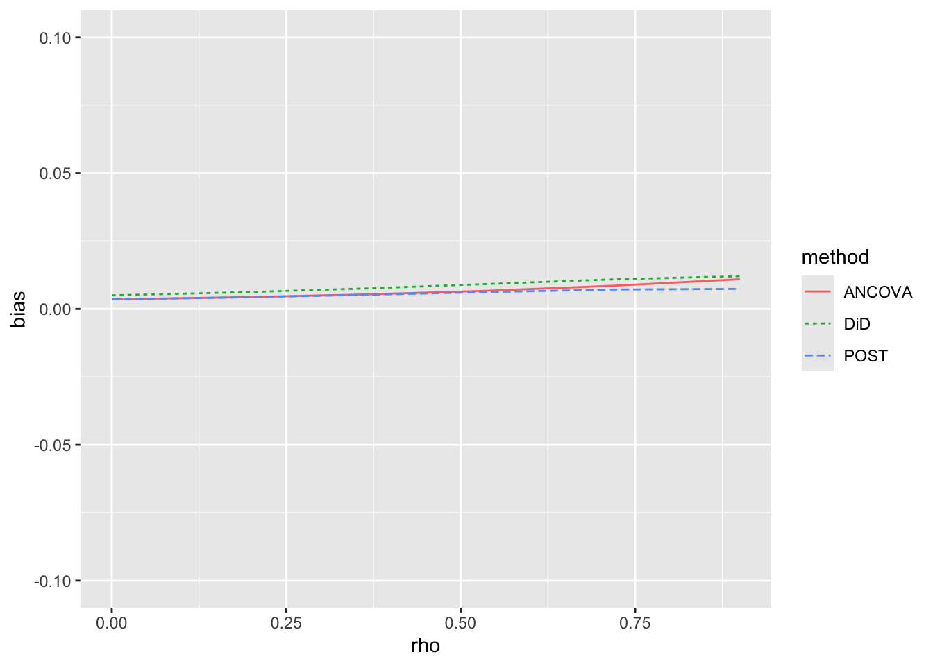
Having confirmed that there is no apparent bias in any of the estimators in this setting, we next consider the empirical standard errors for each method. Because we get essentially identical plots with each value of the true effect, we focus on effect == 0.5 in the following analysis. Here we rearrange the data so that we have a method column and an est column for the estimated causal effect. We then calculate, for each method and value of rho, the standard deviation of est, which is the empirical standard error we seek. Finally, we plot the values for each value of rho in Figure 19.2.
results |>
  filter(effect == 0.5) |>
  pivot_longer(starts_with("est"),
               names_to = "method", values_to = "est") |>
  mutate(method = str_replace(method, "^est.(.*)$", "\\1")) |>
  filter(method != "CHANGE") |>
  group_by(method, rho) |>
  summarize(se = sd(est), .groups = "drop") |>
  ggplot(aes(x = rho, y = se,
             colour = method, linetype = method)) +
  geom_line()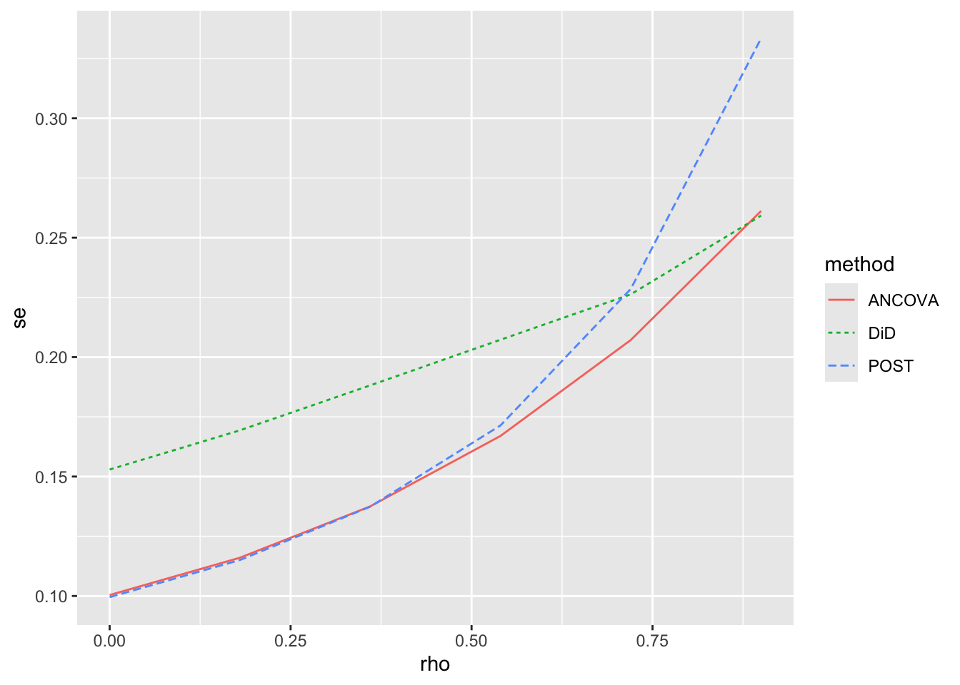
From the above, we can see that for low values of \(\rho\), subtracting pre-treatment outcome values adds noise to our estimation of treatment effects. We actually have lower standard errors when we throw away the pre-treatment data and just compare post-treatment outcomes. But for higher levels of \(\rho\), we see that DiD outperforms POST; by subtracting pre-treatment outcome values, we get a more precise estimate of the treatment effect. However, we see that both DiD and POST are generally outperformed by ANCOVA, which in effect allows for a flexible, data-driven relation between pre- and post-treatment outcome values.
In short, notwithstanding its popularity, it is far from clear that DiD is the best approach to use for all analyses of causal effects based on experimental data. Even in the context of the Reg SHO experiment, the appropriate method may depend on the outcome of interest. For a persistent outcome, DiD may be better than POST, but for a less persistent outcome, POST may be better than DiD. And ANCOVA may be a better choice than either POST or DiD unless there are strong a priori reasons to believe that DiD or POST is more appropriate (and such reasons seem more likely to hold for POST than for DiD).
19.4 Evaluating natural experiments
Because of the plausibly random assignment mechanism used by the SEC, Reg SHO provides a very credible natural experiment. However, in many claimed natural experiments, it will be “nature” who is assigning treatment. In Michels (2017), it was literally nature doing the assignment through the timing of natural disasters. While natural disasters are clearly not completely random, as hurricanes are more likely to strike certain locations at certain times of year, this is not essential for the natural experiment to provide a setting from which causal inferences can be credibly drawn. What is necessary in Michels (2017) is that treatment assignment is as-if random with regard to the timing of the natural disaster before or after the end of the fiscal period and discussion questions in Chapter 17 explored these issues.
More often in claimed natural experiments, it will be economic actors or forces, rather than nature, assigning treatment. While such economic actors and forces are unlikely to act at random, again the critical question is whether treatment assignment is as-if random. To better understand the issues, we consider a well-studied setting, that of brokerage closures as studied in Kelly and Ljungqvist (2012).
Kelly and Ljungqvist (2012, p. 1368) argue that “brokerage closures are a plausibly exogenous source of variation in the extent of analyst coverage, as long as two conditions are satisfied. First, the resulting coverage terminations must correlate with an increase in information asymmetry. … Second, the terminations must only affect price and demand through their effect on information asymmetry.” Interestingly, these are essentially questions 2 and 3 that we ask in evaluating instrumental variables in Section 20.3. The analogue with instrumental variables applies because Kelly and Ljungqvist (2012) are primarily interested in the effects of changes in information asymmetry, not the effects of brokerage closures per se. In principle, brokerage closures could function much like an instrumental variable, except that Kelly and Ljungqvist (2012) estimate reduced-form regressions whereby outcomes are related directly to brokerage closures, such as in Table 3 (Kelly and Ljungqvist, 2012, p. 1391). But the first of the three questions from Section 20.3 remains relevant, and this is the critical question for evaluating any natural experiment: Is treatment assignment (as-if) random?
Like many researchers, Kelly and Ljungqvist (2012) do not address the (as-if) randomness of treatment assignment directly. Instead, Kelly and Ljungqvist (2012) focus on whether brokerage closure-related terminations of analyst coverage “constitute a suitably exogenous shock to the investment environment”. Kelly and Ljungqvist (2012) argue that they do “unless brokerage firms quit research because their analysts possessed negative private information about the stocks they covered.” But this reasoning is incomplete. For sure, brokerage firms not quitting research for the reason suggested is a necessary condition for a natural experiment (otherwise the issues with using brokerage closures as a natural experiment are quite apparent). But it is not a sufficient condition. If the firms encountering brokerage closure-related terminations of analyst coverage had different trends in information asymmetry for other reasons, the lack of private information is inadequate to give us a natural experiment.
In general, we should be able to evaluate the randomness of treatment assignment much as we would do so with an explicitly randomized experiment. Burt (2000) suggest that “statisticians will compare the homogeneity of the treatment group populations to assess the distribution of the pretreatment demographic characteristics and confounding factors.” With explicit randomization, statistically significant differences in pretreatment variables might prompt checks to ensure that, say, there was not “deliberate alteration of or noncompliance with the random assignment code” or any other anomalies. Otherwise, we might have greater confidence that randomization was implemented effectively, and hence that causal inferences might reliably be drawn from the study.
So, a sensible check with a natural experiment would seem to be to compare various pre-treatment variables across treatment groups to gain confidence that “nature” has indeed randomized treatment assignment. In this regard, Table 1 of Kelly and Ljungqvist (2012) is less than assuring. Arguably, one can only encounter brokerage closure-related terminations of analyst coverage if one has analyst coverage in the first place; so the relevant comparison is arguably between the first and third columns of data. There we see that the typical firm in the terminations sample (column 1) is larger, has higher monthly stock turnover, higher daily return volatility, and more brokers covering the stock than does the typical firm in the universe of covered stocks in 2004 (column 3). So clearly “nature” has not randomly selected firms from the universe of covered stocks in 2004.
However, we might come to a similar conclusion if we compared the Reg SHO pilot stocks with the universe of traded stocks or some other broad group. Just as it was essential to correctly identify the population that the SEC considered in randomizing treatment assignment, it is important to identify the population that “nature” considered in assigning treatment in evaluating any natural experiment. While the SEC provided a statement detailing how it constructed the sample, “nature” is not going to do the same and researchers need to consider carefully which units were considered for (as if) random assignment to treatment.
In this regard, even assuming that the controls used in Table 2 of Kelly and Ljungqvist (2012, p. 1388) were the ones “nature” herself considered, it seems that the natural experiment did not assign treatment in a sufficiently random way. Table 2 studies four outcomes: bid-ask spreads, the Amihud illiquidity measure, missing- and zero-return days, and measures related to earnings announcements. In each case, there are pre-treatment differences that sometimes exceed the DiD estimates. For example, pre-treatment bid-ask spreads for treatment and control firms are 1.126 and 1.089, a 0.037 difference that is presumably statistically significant given that the smaller DiD estimate of 0.020 has a p-value of 0.011.10 In light of this evidence, it seems that Kelly and Ljungqvist (2012) need to rely on the parallel trends assumption to draw causal inferences and we evaluate the plausibility of this assumption in the next section.
It is important to recognize that the shortcomings of broker closures as a natural experiment do not completely undermine the ability of Kelly and Ljungqvist (2012) to draw causal inferences. There appears to be an unfortunate tendency to believe, on the one hand, that without some kind of natural experiment, one cannot draw causal inferences. On the other hand, there is an apparent tendency to view natural experiments as giving carte blanche to researchers to draw all kinds of causal inferences, even when the alleged identification strategies do not, properly understood, support such inferences.
In the case of Kelly and Ljungqvist (2012), it seems the authors would like to believe that they have a natural experiment that allows them to draw inferences about the effects of broker closures on information asymmetry (Table 2) and, because broker closures only affect stock prices through their effects on information asymmetry, to conclude from the evidence in Table 3 that increases in information asymmetry reduce stock prices. But Table 2 could have been based on a bullet-proof identification strategy without implying that broker closures only affect stock prices through their effects on information asymmetry. There is really no evidence offered for this claim, one that is arguably very difficult to support.
At the same time, it is conceptually possible that Kelly and Ljungqvist (2012) could provide compelling evidence that the only plausible explanation for the abnormal returns in Table 3 is reductions in information asymmetry, even if the results in Table 2 were irredeemably corrupted (e.g., because of failure of parallel trends). Evidence that firms did not “quit research because their analysts possessed negative private information about the stocks they covered” might support drawing certain inferences from Table 3 even without a credible equivalent of Table 2.
19.5 The parallel trends assumption
Examining the studies of the direct effects of Reg SHO discussed in Section 19.2.3, we see that randomization generally provided balance in pre-treatment outcome values. In such settings, we see that DiD can provide unbiased estimates of causal effects, but that it has little appeal when treatment assignment is random. Indeed, if there is little to distinguish treatment and control observations in terms of pre-treatment outcome values, DiD will differ little from simply comparing differences in post-treatment means (the POST estimator discussed above).
But in many settings, such as that in Kelly and Ljungqvist (2012), differences in pre-treatment outcome values exist, suggesting that random assignment is not an appropriate assumption. In such settings, it will therefore be necessary to rely on a different assumption to justify the use of DiD for causal inferences. This parallel trends assumption posits that, but for treatment, the expected change in the outcome variable for the treated observations would equal that for control observations. Using this assumption, we can attribute any difference in the change in the outcome variable between the treated and control observations to a treatment effect and random variation and use standard tools of statistical inference to evaluate the null hypothesis that any difference is due to random variation.
That DiD can be predicated on an assumption other than (as-if) random assignment may explain its popularity. Cunningham (2021, p. 406) suggests that DiD “has become the single most popular research design in the quantitative social sciences” and Armstrong et al. (2022, p. 4) find rapid “increase in [the number of] papers using quasi-experimental methods to draw causal inferences, that more than 75% of such papers use variations of the classic difference-in-differences design.”
Arguably DiD is more often used in settings that without (as-if) random assignment of treatment. For example, one of the most highly cited papers using DiD is Card and Krueger (1994), which compares the change in employment in the fast-food industry in New Jersey and Philadelphia before and after an increase in the minimum wage in New Jersey. In this case, treatment assignment was very clearly non-random—it was a function of being located in New Jersey.
Unlike the assumption of random assignment, the parallel trends assumption is not implied by a reasonable description of a physical or economic process and thus is of a fundamentally different nature. Random assignment is widely regarded as a reasonable description of, say, a coin toss or the generation of pseudo-random numbers using a computer. In contrast, it is difficult to think of a mechanism for imposing parallel trends on the data. Because DiD is—unlike instrumental variables or regression discontinuity designs—generally not predicated on “as-if random variation in the explanatory variable of interest”, it is not correct to consider DiD as a quasi-experimental method (Armstrong et al., 2022, p. 3).11
Instead the basis for the parallel trends assumption appears to be that it is the assumption that is necessary (and sufficient) for the DiD estimator to provide an unbiased estimator of the causal effect of treatment. But “assuming a can-opener” seems to be a weak foundation for an approach as widespread as DiD.
On the one hand, as discussed above, there is no obvious economic basis for the parallel trends assumption with general applicability. On the other hand, there are often reasons to believe that the parallel trends assumption will not hold for various outcomes. The parallel trends assumption will be dubious when the outcome variable tends to be mean-reverting. For example, it is well known that accounting-based measures of operating performance tend to revert towards the mean. So if treatment and control observations have different levels of pre-treatment operating performance, the parallel trends assumption will be a highly dubious basis for causal inference.
Another reason to doubt the parallel trends assumption is the fact that the measurement of outcomes is often arbitrary. For example, Li et al. (2018) examine the effect of legal changes on disclosure of customer identities using a variant of DiD.12 One primary outcome measure considered by Li et al. (2018) is \(\texttt{ratio}\), the proportion of significant customers whose identities are not disclosed. But if the parallel trends assumption holds in \(\texttt{ratio}\) then, so long as there are pre-treatment differences between treatment and control observations, it is not mathematically possible for parallel trends to hold in \(\log(1 + \texttt{ratio})\), which is the measure used in the regression analysis in Li et al. (2018).
The apparent flimsiness of the parallel trends assumption underlying DiD analysis in non-randomized settings is perhaps reinforced by the treatment of DiD in textbooks. Imbens and Rubin (2015), a significant recent tome on causal inference, buries DiD in endnotes, merely noting that DiD is “widely used” (2015, p. 44) before directing the reader to Angrist and Pischke (2008). While Angrist and Pischke (2008) discuss DiD and its assumptions, and relate it to fixed-effects regressions and panel data methods, they do little to justify the parallel trends assumption. Cunningham (2021) is much more cautious in discussing the parallel trends assumption, which he notes “is by definition untestable since we cannot observe this counterfactual conditional expectation [of post-treatment outcomes absent treatment]”.
Two popular approaches to address the parallel trends assumption are discussed by Cunningham (2021) and Huntington-Klein (2021). The first approach compares the trends in pre-treatment outcome values for treatment and control observations. If these trends are similar before treatment, it is perhaps reasonable to assume they are similar after treatment. But Cunningham (2021, p. 426) notes that “pre-treatment similarities are neither necessary nor sufficient to guarantee parallel counterfactual trends” and this seems an especially dubious assumption if treatment is endogenously selected.
The second approach is the placebo test, variants of which are discussed by Cunningham (2021) and Huntington-Klein (2021). One placebo test involves evaluating the treatment effect in a setting where prior beliefs hold that there should be no effect. Another approach involves a kind of random assignment of a pseudo-treatment. In either case, not finding an effect is considered as providing support for the parallel trends assumption in the analysis of greater interest to the researcher. Of course, one might be sceptical of such placebo tests in light of the concerns raised at the start of this chapter. If applying DiD to state-level data on spending on science, space, and technology provides evidence of an effect on suicides by hanging, strangulation, and suffocation, not finding an effect on deaths by drowning after falling out of a canoe or kayak may provide limited assurance.
To illustrate, we now apply a kind of placebo test to evaluate the parallel trends assumption for bid-ask spreads, one of the variables considered in the DiD analysis of Table 2 of Kelly and Ljungqvist (2012) (we choose spreads in part because it is easy to calculate).
We first create the data set spreads, which contains data on the average spread for stocks over three-month periods—aligning with one measure used Table 2 of Kelly and Ljungqvist (2012)—for a sample period running from Q1, 2001 (the first quarter of 2001) to Q1, 2008, which is the sample period in Kelly and Ljungqvist (2012). We will conduct a study of a pseudo-treatment that we will assume applies for periods beginning in Q1, 2004, which is roughly halfway through the sample period and we code post accordingly.
db <- dbConnect(RPostgres::Postgres(), bigint = "integer")

dsf <- tbl(db, Id(schema = "crsp", table = "dsf"))

spreads <-
  dsf |>
  mutate(spread = 100 * (ask - bid) / ((ask + bid) / 2),
         quarter = as.Date(floor_date(date, 'quarter'))) |>
  group_by(permno, quarter) |>
  summarize(spread = mean(spread, na.rm = TRUE), .groups = "drop") |>
  mutate(post = quarter >= "2004-01-01") |>
  filter(!is.na(spread),
         between(quarter, "2000-01-01", "2008-01-01")) |>
  collect()

dbDisconnect(db)
db <- dbConnect(duckdb::duckdb())
dsf <- load_parquet(db, schema = "crsp", table = "dsf")
spreads <-
dsf |>
mutate(spread = 100 * (ask - bid) / ((ask + bid) / 2),
quarter = as.Date(floor_date(date, 'quarter'))) |>
group_by(permno, quarter) |>
summarize(spread = mean(spread, na.rm = TRUE), .groups = "drop") |>
mutate(post = quarter >= "2004-01-01") |>
filter(!is.na(spread),
between(quarter, "2000-01-01", "2008-01-01")) |>
collect()
dbDisconnect(db)We now randomize treatment assignment. Because we want to evaluate the parallel trends assumption and completely randomized treatment assignment implies a trivial version of the parallel trends assumption, we specify a small difference in the probability of receiving treatment for observations whose pre-treatment spread exceeds the median (\(p = 0.55\)) from those whose pre-treatment spread is below the median (\(p = 0.45\)). This ensures that we have pre-treatment differences and thus need to rely on the parallel trends assumption in a meaningful way.13
set.seed(2021)

treatment <-
  spreads |>
  filter(!post) |>
  group_by(permno) |>
  summarize(spread = mean(spread, na.rm = TRUE), .groups = "drop") |>
  mutate(treat_prob = if_else(spread > median(spread), 0.55, 0.45),
         rand = runif(n = nrow(pick(everything()))),
         treat = rand < treat_prob) |>
  select(permno, treat)
Obviously the null hypothesis of zero treatment effect holds with this “treatment”, but the question is whether the parallel trends assumption holds for spread. If we find evidence of a “treatment effect”, the only sensible interpretation is a failure of the parallel trends assumption for spread.
Merging in the treatment data set, we estimate a DiD regression (and cluster standard errors by permno for reasons that will be apparent after reading the discussion below). Results are reported in Table 19.2.
reg_data <-
  spreads |>
  inner_join(treatment, by = "permno")

fm <- feols(spread ~ post * treat, vcov = ~ permno, data = reg_data)modelsummary(fm,
estimate = "{estimate}{stars}",
gof_map = c("nobs"),
stars = c('*' = .1, '**' = 0.05, '***' = .01))| (1) | |
|---|---|
| (Intercept) | 2.830*** |
| (0.049) | |
| postTRUE | -2.130*** |
| (0.044) | |
| treatTRUE | 0.489*** |
| (0.077) | |
| postTRUE × treatTRUE | -0.343*** |
| (0.069) | |
| Num.Obs. | 220822 |
Because we find a statistically significant effect of \(-0.343\) with a t-statistic of \(-4.96\) with this meaningless “treatment”, we can conclude with some confidence that the parallel trends assumption simply does not hold for spread in this sample. Given that we might have passed this placebo test even if the parallel trends assumption did not hold for a particular treatment, say due to endogenous selection, it seems reasonable to view this test as being better suited to detecting a failure of parallel trends (as it does here) than it is to validation of that assumption.
Cunningham (2021) and Huntington-Klein (2021) provide excellent pathways to a recent literature examining DiD. However, it is important to recognize that some variant of the scientifically flimsy parallel trends assumption imbues all of these treatments. It would seem to be productive for researchers to discard the “quasi-experimental” pretence attached to DiD and to apply techniques appropriate to what some call interrupted time-series designs (e.g., Shadish et al., 2002).14
While a randomized experiment provides a sound basis for attributing observed differences in outcomes to either treatment effects or sampling variation, without such randomization, it is perhaps more appropriate to take a more abductive approach of identifying causal mechanisms, deeper predictions about the timing and nature of causal effects, explicit consideration of alternative explanations, and the like (Armstrong et al., 2022; Heckman and Singer, 2017). Some evidence of this is seen in the discussion of specific papers in Cunningham (2021), perhaps reflecting reluctance to lean too heavily on the parallel trends assumption.
19.6 Indirect effects of Reg SHO
The early studies of Reg SHO discussed above can be viewed as studying the more direct effects of Reg SHO. As a policy change directly affecting the ability of short-sellers to trade in securities, the outcomes studied by these earlier studies are more closely linked to the Reg SHO pilot than are the outcomes considered in later studies. Black et al. (2019, pp. 2–3) point out that “despite little evidence of direct impact of the Reg SHO experiment on pilot firms, over 60 papers in accounting, finance, and economics report that suspension of the price tests had wide-ranging indirect effects on pilot firms, including on earnings management, investments, leverage, acquisitions, management compensation, workplace safety, and more.”
One indirect effect of short-selling that has been studied in subsequent research is that on earnings management. To explore this topic, we focus on Fang et al. (2016, p. 1251), who find “that short-selling, or its prospect, curbs earnings management.”
19.6.1 Earnings management after Dechow et al. (1995)
In Chapter 16, we saw that early earnings management research used firm-specific regressions in estimating standard models such as the Jones (1991) model. Fang et al. (2016) apply subsequent innovations in measurement of earnings management, such the performance-matched discretionary accruals measure developed in Kothari et al. (2005).
Kothari et al. (2005) replace the firm-specific regressions seen in Dechow et al. (1995) with regressions by industry-year, where industries are defined as firms grouped by two-digit SIC codes. Kothari et al. (2005) also add an intercept term to the Jones Model and estimate discretionary accruals under the Modified Jones Model by applying the coefficients from the Jones Model to the analogous terms of the Modified Jones Model.15
To calculate performance-matched discretionary accruals, Kothari et al. (2005, p. 1263) “match each sample firm with the firm from the same fiscal year-industry that has the closest return on assets as the given firm. The performance-matched discretionary accruals … are then calculated as the firm-specific discretionary accruals minus the discretionary accruals of the matched firm.” This is the primary measure of earnings management used by Fang et al. (2016), but note that Fang et al. (2016) use the 48-industry Fama-French groupings, rather than the two-digit SIC codes used in Kothari et al. (2005).
19.6.2 FHK: Data steps
To construct measures of discretionary accruals, Fang et al. (2016) obtain data primarily from Compustat, along with data on Fama-French industries from Ken French’s website and data on the SHO pilot indicator from the SEC’s website. The following code is adapted from code posted by the authors of Fang et al. (2016), which was used to produce the results found in Tables 15 and 16 of Fang et al. (2019). The bulk of the Compustat data used in Fang et al. (2016) come from comp.funda. Following Fang et al. (2019), the code below collects data from that table for fiscal years between 1999 and 2012, excluding firms with SIC codes between 6000 and 6999 or between 4900 and 4949.
db <- dbConnect(RPostgres::Postgres(), bigint = "integer")

funda <- tbl(db, Id(schema = "comp", table = "funda"))

compustat_annual <-
  funda |>
  filter(indfmt == 'INDL', datafmt == 'STD', popsrc == 'D', consol == 'C',
         between(fyear, 1999, 2012),
         !(between(sich, 6000, 6999) | between(sich, 4900, 4949))) |>
  select(gvkey, fyear, datadate, fyr, sich, dltt, dlc, seq,
         oibdp, ib, ibc, oancf, xidoc, at, ppegt, sale,
         rect, ceq, csho, prcc_f) |>
  mutate(fyear = as.integer(fyear)) |>
  collect()

dbDisconnect(db)
db <- dbConnect(duckdb::duckdb())
funda <- load_parquet(db, schema = "comp", table = "funda")
compustat_annual <-
funda |>
filter(indfmt == 'INDL', datafmt == 'STD', popsrc == 'D', consol == 'C',
between(fyear, 1999, 2012),
!(between(sich, 6000, 6999) | between(sich, 4900, 4949))) |>
select(gvkey, fyear, datadate, fyr, sich, dltt, dlc, seq,
oibdp, ib, ibc, oancf, xidoc, at, ppegt, sale,
rect, ceq, csho, prcc_f) |>
mutate(fyear = as.integer(fyear)) |>
collect()
dbDisconnect(db)Some regressions in Fang et al. (2019) consider controls for market-to-book, leverage, and return on assets, which are calculated as mtob, leverage, and roa, respectively, in the following code:
controls_raw <-
  compustat_annual |>
  group_by(gvkey) |>
  arrange(fyear) |>
  mutate(lag_fyear = lag(fyear),
         mtob = if_else(lag(ceq) != 0,
                        lag(csho) * lag(prcc_f) / lag(ceq), NA),
         leverage = if_else(dltt + dlc + seq != 0,
                            (dltt + dlc) / (dltt + dlc + seq), NA),
         roa = if_else(lag(at) > 0, oibdp / lag(at), NA)) |>
  filter(fyear == lag(fyear) + 1) |>
  ungroup() |>
  select(gvkey, datadate, fyear, at, mtob, leverage, roa)
Following Fang et al. (2019), we create controls_filled, which uses fill() to remove many missing values for the controls.
Following Fang et al. (2019), we create controls_fyear_avg, which calculates averages of controls by fiscal year.
Like Fang et al. (2019), we use values from controls_fyear_avg to replace missing values for controls.
There are multiple steps in the code above and the reasons for the steps involved in calculating controls_filled from controls_raw and df_controls from controls_filled are explored in the exercises below.
As discussed above, FHK estimate discretionary-accrual models by industry and year, where industries are based on the Fama-French 48-industry grouping. To create these industries here, we use get_ff_ind(), introduced in Chapter 9 and provided by the farr package.
ff_data <- get_ff_ind(48)We now create functions to compile the data we need to estimate performance-matched discretionary accruals. We use a function to compile the data because (i) doing so is easy in R and (ii) it allows us to re-use code much easily, which will be important for completing the exercises in this chapter.
The first function we create is get_das(), which takes as its first argument (compustat) a data set derived from Compustat with the requisite data. The second argument (drop_extreme) allows to easily tweak the handling of outliers in a way examined in the exercises.
Within get_das(), the first data set we compile is for_disc_accruals, which contains the raw data for estimating discretionary-accruals models. Following FHK, we require each industry-year to have at least 10 observations for inclusion in our analysis and impose additional data requirements, some of which we explore in the exercises below.
Following FHK, we estimate discretionary-accrual models by industry and year and store the results in the data frame fm_da. We then merge the underlying data (for_disc_accruals) with fm_da to use the estimated models to calculate non-discretionary accruals (nda). Because the coefficient on sale_c_at is applied to salerect_c_at, we cannot use predict() or residuals() in a straightforward fashion and need calculate nda “by hand”. We then calculate discretionary accruals (da = acc_at - nda) and return the data.
get_das <- function(compustat, drop_extreme = TRUE) {

  for_disc_accruals <-
    compustat |>
    inner_join(ff_data,
               join_by(between(sich, sic_min, sic_max))) |>
    group_by(gvkey, fyr) |>
    arrange(fyear) |>
    filter(lag(at) > 0) |>
    mutate(lag_fyear = lag(fyear),
           acc_at = (ibc - (oancf - xidoc)) / lag(at),
           one_at = 1 / lag(at),
           ppe_at = ppegt / lag(at),
           sale_c_at = (sale - lag(sale)) / lag(at),
           salerect_c_at = ((sale - lag(sale)) -
                              (rect - lag(rect))) / lag(at)) |>
    ungroup() |>
    mutate(keep = case_when(drop_extreme ~ abs(acc_at) <= 1,
                            .default = TRUE)) |>
    filter(lag_fyear == fyear - 1,
           keep,
           !is.na(salerect_c_at), !is.na(acc_at), !is.na(ppe_at)) |>
    group_by(ff_ind, fyear) |>
    mutate(num_obs = n(), .groups = "drop") |>
    filter(num_obs >= 10) |>
    ungroup()

  fm_da <-
    for_disc_accruals |>
    group_by(ff_ind, fyear) |>
    do(model = tidy(lm(acc_at ~ one_at + sale_c_at + ppe_at, data = .))) |>
    unnest(model) |>
    select(ff_ind, fyear, term, estimate) |>
    pivot_wider(names_from = "term", values_from = "estimate",
                names_prefix = "b_")

  for_disc_accruals |>
    left_join(fm_da, by = c("ff_ind", "fyear")) |>
    mutate(nda = `b_(Intercept)` + one_at * b_one_at + ppe_at * b_ppe_at +
                   salerect_c_at * b_sale_c_at,
           da = acc_at - nda) |>
    select(gvkey, fyear, ff_ind, acc_at, da)
}
The next step in the data preparation process is to match each firm with another based on performance. Following FHK, we calculate performance as lagged “Income Before Extraordinary Items” (ib) divided by lagged “Total Assets” (at) and perf_diff, the absolute difference between performance for each firm-year and each other firm-year in the same industry. We then select the firm (gvkey_other) with the smallest value of perf_diff. We rename the variable containing the discretionary accruals of the matching firm as da_other and calculate performance-matched discretionary accruals (da_adj) as the difference between discretionary accruals for the target firm (da) and discretionary accruals for the matched firm (da_other), and return the results. Note that get_pm() includes the argument pm_lag with default value TRUE. If pm_lag is set to FALSE, then performance for matching is calculated using contemporary values of ib and at (this option is examined in the exercises below).
get_pm <- function(compustat, das, pm_lag = TRUE, drop_extreme = TRUE) {

  das <- get_das(compustat, drop_extreme = drop_extreme)

  perf <-
    compustat |>
    group_by(gvkey) |>
    arrange(fyear) |>
    mutate(ib_at =
      case_when(pm_lag ~ if_else(lag(at) > 0, lag(ib) / lag(at), NA),
                .default = if_else(at > 0, ib / at, NA))) |>
    ungroup() |>
    inner_join(das, by = c("gvkey", "fyear")) |>
    select(gvkey, fyear, ff_ind, ib_at)

  perf_match <-
    perf |>
    inner_join(perf, by = c("fyear", "ff_ind"),
               suffix = c("", "_other")) |>
    filter(gvkey != gvkey_other) |>
    mutate(perf_diff = abs(ib_at - ib_at_other)) |>
    group_by(gvkey, fyear) |>
    filter(perf_diff == min(perf_diff)) |>
    select(gvkey, fyear, gvkey_other)

  perf_matched_accruals <-
    das |>
    rename(gvkey_other = gvkey,
           da_other = da) |>
    select(fyear, gvkey_other, da_other) |>
    inner_join(perf_match, by = c("fyear", "gvkey_other")) |>
    select(gvkey, fyear, gvkey_other, da_other)

  das |>
    inner_join(perf_matched_accruals, by = c("gvkey", "fyear")) |>
    mutate(da_adj = da - da_other) |>
    select(gvkey, fyear, acc_at, da, da_adj, da_other, gvkey_other)
}
The final step is performed in get_pmdas(). This function gets the needed data using get_pm(), then filters duplicate observations based on (gvkey, fyear) (the rationale for this step is explored in the discussion questions).
get_pmdas <- function(compustat, pm_lag = TRUE, drop_extreme = TRUE) {

  get_pm(compustat,
         pm_lag = pm_lag,
         drop_extreme = drop_extreme) |>
    group_by(gvkey, fyear) |>
    filter(row_number() == 1) |>
    ungroup()
}
Finally, we simply pass the data set compustat_annual to get_pmdas() and store the result in pmdas.
pmdas <- get_pmdas(compustat_annual)The remaining data set used by FHK is sho_data, which we discussed in Section 19.2.1.
The final sample sho_accruals is created in the following code and involves a number of steps. We first merge data from FHK’s sho_data with fhk_firm_years to produce the sample firm-years and treatment indicator for FHK. As fhk_firm_years can contain multiple years for each firm, so we expect each row in sho_data to match multiple rows in fhk_firm_years. At the same time, some gvkey values link with multiple PERMNOs, so some rows in fhk_firm_years will match multiple rows in sho_data. As such, we set relationship = "many-to-many" in this join below. We then merge the resulting data set with df_controls, which contains data on controls. The final data merge brings in data on performance-matched discretionary accruals from pm_disc_accruals_sorted. Finally, following FHK, we winsorize certain variables using the winsorize() function from the farr package to do this here.16
win_vars <- c("at", "mtob", "leverage", "roa", "da_adj", "acc_at")

sho_accruals <-
  sho_data |>
  inner_join(fhk_firm_years,
             by = "gvkey",
             relationship = "many-to-many") |>
  select(gvkey, datadate, pilot) |>
  mutate(fyear = year(datadate) - (month(datadate) <= 5)) |>
  left_join(df_controls, by = c("gvkey", "fyear")) |>
  left_join(pmdas, by = c("gvkey", "fyear")) |>
  group_by(fyear) |>
  mutate(across(all_of(win_vars),
                \(x) winsorize(x, prob = 0.01))) |>
  ungroup()
19.6.3 Discussion questions and exercises
- What would be the effect of replacing the code that creates
ff_dataabove with the following code? What changes would we need to make to the code creatingfor_disc_accrualsinget_das()to use this modified version offf_data?
What issue is
filter(row_number() == 1)addressing in the code above? What assumptions are implicit in this approach? Do these assumptions hold in this case? What would be an alternative approach to address the issue?Why is
filter(fyear == lag(fyear) + 1)required in the creation ofcontrols_raw?Does the argument for using
salerect_c_at * b_sale_c_atin creating non-discretionary accruals make sense to you? How do Kothari et al. (2005) explain this?Does the code above ensure that a performance-matched control firm is used as a control just once? If so, which aspect of the code ensures this is true? If not, how might you ensure this and does this cause problems? (Just describe the approach in general; no need to do this.)
What are FHK doing in the creation of
controls_filled? (Hint: The key “verb” isfill().) Does this seem appropriate? Does doing this make a difference?What are FHK doing in the creation of
df_controlsfromcontrols_fyear? Does this seem appropriate? Does doing this make a difference?
19.6.4 FHK: Regression analysis
FHK consider a number of regression specifications including: with and without controls, with and without firm fixed effects, and with standard errors clustered by firm alone and clustered by firm and year. We make a small function (reg_year_fe()) that calculates variables used in the regression (like during and post) and allows us to specify each of these different options, to change the dependent variable from the default (dv = "da_adj") and to supply a different data set. This function returns a fitted model that is estimated using feols() from the fixest package.
ctrls_list <- c("log(at)", "mtob", "roa", "leverage")

reg_year_fe <- function(df, dv = "da_adj",
                        controls = TRUE, firm_fe = FALSE, cl_2 = TRUE,
                        vcov = NULL) {
  df <-
    df |>
    mutate(year = year(datadate),
           during = year %in% c(2005, 2006, 2007),
           post = year %in% c(2008, 2009, 2010))

  model <- str_c(dv, " ~ pilot * (during + post) ",
                 if_else(controls,
                         str_c(" + ", str_c(ctrls_list,
                                            collapse = " + ")), ""),
                    if_else(firm_fe, "| gvkey + year ", "| year "))
  if (is.null(vcov)) {
    vcov = as.formula(if_else(!cl_2, "~ gvkey ", "~ year + gvkey"))
  }

  feols(as.formula(model),
        vcov = vcov,
        notes = FALSE,
        data = df)
}
To facilitate the output of variations, we next make a function that runs regressions with and without controls and with and without firm fixed effects and returns a nicely formatted regression table.
make_reg_table <- function(df, dv = "da_adj", cl_2 = TRUE) {
  omit <- str_c("^(", str_c(str_replace_all(c("during", "post", ctrls_list),
                                            "[()]", "."),
                            collapse="|"), ")")

  run_reg <- function(controls, firm_fe) {
    reg_year_fe(df, dv = dv, controls = controls, firm_fe = firm_fe,
                cl_2 = cl_2)
  }

  params <- tibble(controls = c(FALSE, TRUE, FALSE, TRUE),
                   firm_fe = c(FALSE, FALSE, TRUE, TRUE))

  fms <- pmap(params, run_reg)

  notes <- tribble(~term,  ~`1`,  ~`2`, ~`3`, ~`4`,
                   "Firm FEs", "No", "No", "Yes", "Yes",
                   "Controls", "No", "Yes", "No", "Yes")

  modelsummary(fms,
               estimate = "{estimate}{stars}",
               gof_map = "nobs",
               stars = c('*' = .1, '**' = 0.05, '***' = .01),
               coef_omit = str_c(str_replace_all(ctrls_list, "[()]", "."),
                                 collapse = "|"),
               add_rows = notes)
}
We now use this function with our version of FHK’s data set (sho_accruals) to create the regression results reported in Table 19.3.
make_reg_table(sho_accruals)| (1) | (2) | (3) | (4) | |
|---|---|---|---|---|
| pilotTRUE | 0.000 | 0.000 | ||
| (0.004) | (0.004) | |||
| pilotTRUE × duringTRUE | -0.010** | -0.010** | -0.014** | -0.014** |
| (0.004) | (0.004) | (0.005) | (0.005) | |
| pilotTRUE × postTRUE | 0.009** | 0.008** | 0.005 | 0.005 |
| (0.004) | (0.004) | (0.004) | (0.004) | |
| Num.Obs. | 19616 | 19616 | 19616 | 19616 |
| Firm FEs | No | No | Yes | Yes |
| Controls | No | Yes | No | Yes |
We next create a function that allows us to plot by-year coefficients for the treatment and control firms. (We leave the details of what this function is doing as an exercise for the reader below.)
plot_coefficients <- function(model) {
  tibble(name = names(model$coefficients),
         value = as.vector(model$coefficients)) |>
  filter(str_detect(name, "^year.")) |>
  separate(name, into = c("year", "pilot"), sep = ":", fill = "right") |>
  mutate(year = as.integer(str_replace(year, "^year", "")),
         pilot = coalesce(pilot == "pilotTRUE", FALSE)) |>
  ggplot(aes(x = year, y = value,
             linetype = pilot, color = pilot)) +
  geom_line() +
  scale_x_continuous(breaks = 2000:2012L) +
  geom_rect(xmin = 2005, xmax = 2007, ymin = -Inf, ymax = Inf,
              color = NA, alpha = 0.01) +
  theme_bw()
}
To produce Figure 19.3, we estimate one of the models above by year and feed the fitted model to plot_coefficients().
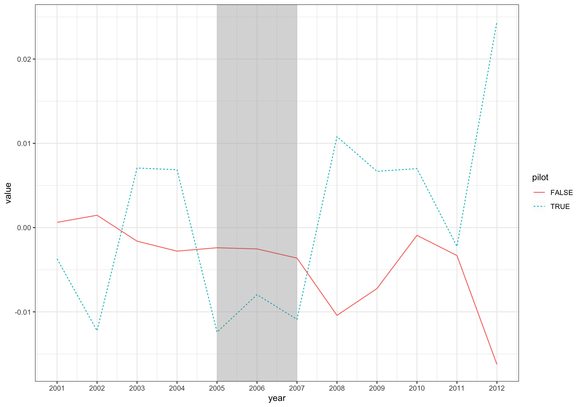
19.6.5 Exercises
- In words, how does
sho_accruals_alt(defined below) differ fromsho_accruals? Does usingsho_accruals_altin place ofsho_accrualsaffect the regression results?
firm_years <-
  controls_raw |>
  select(gvkey, datadate, fyear)

sho_accruals_alt <-
  sho_r3000_gvkeys |>
  inner_join(firm_years, by = "gvkey") |>
  left_join(df_controls, by = c("gvkey", "fyear")) |>
  left_join(pmdas, by = c("gvkey", "fyear")) |>
  group_by(fyear) |>
  mutate(across(all_of(win_vars), winsorize, prob = 0.01)) |>
  ungroup()
In an online appendix, BDLYY say “FHK winsorize covariates for their covariate balance table at 1/99%. We inferred that they also winsorized accruals at this level. Whether they winsorize across sample years or within each year, they do not specify.” The code above winsorized within each year. How would you modify the code to winsorize “across sample years”? Does doing so make a difference?
How would you modify the code to winsorize at the 2%/98% level? Does this make a difference to the results? (Hint: With the
farrpackage loaded, type? winsorizein the R console to get help on this function.)How would you modify the code to not winsorize at all? Does this make a difference to the results?
Some of the studies discussed by BDLYY exclude 2004 data from the sample. How would you modify the code above to do this here? Does excluding 2004 here make a significant difference?
What is the range of values for
yearinsho_accruals? Does this suggest any issues with the codepost = year %in% c(2008, 2009, 2010)above? If so, does fixing any issue have an impact on the results reported above?Would it make sense, in creating
perfabove, if we instead calculatedib_atasif_else(at > 0, ib / at, NA))? What is the effect on the regression results if we use this modified calculation ofib_at? What do Kothari et al. (2005) recommend on this point? (Hint: Usepm_lag = FALSEwhere applicable.)Fang et al. (2019, p. 10) follow Fang et al. (2016), who “exclude observations for which the absolute value of total accruals-to-total assets exceeds one. This is a standard practice in the accounting literature because firms with such high total accruals-to-total assets are often viewed as extreme outliers. Nonetheless, the FHK results are robust to winsorizing the accrual measures at the 1% and 99% levels instead of excluding extreme outliers.” Does this claim hold up in the reproduction above? What happens if the
filteronabs(acc_at) <= 1is removed from the code above? (Hint: Usedrop_extreme = FALSEwhere applicable.)Explain what each line of the function
plot_coefficients()before the line starting withggplot()is doing. (Hint: It may be helpful to store the model that is fed to the function above in the variablemodeland then run the function line by line.)
19.7 Statistical inference
One point of difference between FHK and BDLYY concerns clustered standard errors. Fang et al. (2016) generally use “standard errors clustered by year and firm” (2016, p. 1269), while Black et al. (2019) advocate the use of standard errors clustered by firm. Citing Cameron et al. (2008), Black et al. (2019, p. 30) suggest that “clustered standard errors with a small number of clusters can be downward biased.” In the context of FHK, there are thousands of firms, but a relatively small number of years, so clustering by year (or firm and year) may result in problematic standard error estimates (see Section 5.6.6).
One approach to determining the appropriate clustering is more empirical. In this regard, it is useful to note that cluster-robust standard errors are a generalization of an idea from White (1980). White (1980) provides not only an estimator of standard errors that is robust to heteroskedasticity, but also a test of a null hypothesis of homoskedasticity. Intuitively, if the covariance matrix assuming heteroskedasticity is sufficiently different from that assuming homoskedasticity, then we may reject the null hypothesis of homoskedasticity. With a little algebra, it would be possible to develop a test analogous to that of White (1980) of the null hypothesis of no clustering on variable \(g\). In practice, many researchers will, lacking a formally derived test, compare standard errors with and without clustering on variable \(g\) and elect to cluster on variable \(g\) when the standard errors when doing so seem significantly higher than when not doing so. This heuristic breaks down in the case of Fang et al. (2016) because standard errors are generally lower when clustering on firm and year than when clustering firm alone. However, if clustering on firm alone is appropriate, standard errors clustering on firm and year will provide noisier estimates than clustering on firm alone, and thus could be lower or higher in any given data set.
A more theoretical approach can be used in the setting of FHK because of our deeper understanding of the assignment mechanism. In this regard, it is important to note that cluster-robust standard errors address correlation in both \(X\) and \(\epsilon\) across units within clusters. To explore this (slightly) more formally, recall from Chapter 5 that the cluster-robust covariance matrix is estimated using the following expression:
\[ \hat{V}(\hat{\beta}) = (X'X)^{-1} \hat{B} (X'X)^{-1} \text{, where } \hat{B} = \sum_{g=1}^G X'_g u_g u'_g X_g \]
where the observations grouped into \(G\) clusters of \(N_g\) observations for \(g\) in \({1, \dots, G}\), \(X_g\) is the \(N_g \times K\) matrix of regressors, and \(u_g\) is the \(N_g\)-vector of residuals for cluster \(g\).
If we have a single regressor, demeaned \(x\) with no constant term and two firms (\(i\) and \(j\)) in a cluster, then the contribution of that cluster to \(\hat{B}\) will be
\[ \begin{aligned} \begin{bmatrix} x_i & x_j \end{bmatrix} \begin{bmatrix} u_i \\ u_j \end{bmatrix} \begin{bmatrix} u_i & u_j \end{bmatrix} \begin{bmatrix} x_i \\ x_j \end{bmatrix} &= \begin{bmatrix} x_i & x_j \end{bmatrix} \begin{bmatrix} u_i^2 & u_i u_j \\ u_i u_j & u_j^2 \end{bmatrix} \begin{bmatrix} x_i \\ x_j \end{bmatrix} \\ &= \begin{bmatrix} x_i & x_j \end{bmatrix} \begin{bmatrix} x_i u_i^2 + x_j u_i u_j \\ x_i u_i u_j + x_j u_j^2 \end{bmatrix} \\ &= \begin{bmatrix} x_i^2 u_i^2 + x_i x_j u_i u_j \\ x_i x_j u_i u_j + x_j^2 u_j^2 \end{bmatrix} \end{aligned} \]
Now, if \(x_i\) and \(x_j\) are uncorrelated then, even if \(\epsilon_i\) and \(\epsilon_j\) are correlated, this resolves in expectation to
\[ \begin{bmatrix} x_i^2 \sigma_i^2 \\ x_j^2 \sigma_j^2 \end{bmatrix} \]
which is the expectation of the analogous component of the heteroskedasticity-robust estimator from White (1980). In the setting of Fang et al. (2016), the “\(x\)” of primary interest is the Reg SHO pilot indicator, which is assumed to be randomly assigned, and thus (in expectation) uncorrelated across firms. For this reason, we do not expect cross-sectional dependence to affect standard error estimates on average. On the other hand, the Reg SHO pilot indicator is perfectly correlated over time within firm, so any serial dependence in errors within firm over time will lead to effects of time-series dependence on standard error estimates. This (somewhat loose) theoretical analysis suggests we should cluster by firm (time-series dependence), but not by year (cross-sectional dependence), as suggested by Black et al. (2019, p. 12).
However, the assumed random assignment of treatment allows us to adopt an alternative approach to statistical inference that is agnostic to the form of clustering in the data. This approach is known as randomization inference and builds on the Fisher sharp null hypothesis of no effect of any kind. This is a “sharp null” because it is more restrictive that a null hypothesis of zero mean effect, which could be true even if half the observations had a treatment effect of \(+1\) and half the observations had a treatment effect of \(-1\), in which case the Fisher sharp null would not be true even though null hypothesis of zero mean effect is true.
Under the Fisher sharp null hypothesis and with random assignment to treatment, in principle we can evaluate the distribution of any given test statistic by considering all possible assignments. Focusing on the 2954 firms that the SEC focused on as its initial sample, if assignment to treatment were purely random, then any other assignment of treatment to 985 was as likely as the one chosen. Given that the Fisher sharp null implies that there was no impact of treatment assignment on outcomes, we know what the distribution of the test statistic would have been if the SEC had chosen any one of those alternative assignments because the outcomes would have been exactly the same. With smaller samples, we might proceed to calculate the test statistic for every possible assignment and thereby construct the exact distribution of the test statistic under the Fisher sharp null.17 But in our case, there will be a huge number of ways to choose 985 treatment firms from 2954 possibilities; so a more feasible approach is to draw a random sample of possible assignments and use the empirical distribution of the test statistic for that random sample as an approximation for the exact distribution.
get_coef_rand <- function(i) {
  treatment <-
    sho_accruals |>
    select(gvkey, pilot) |>
    distinct() |>
    mutate(pilot = sample(pilot, size = length(pilot), replace = FALSE))

  reg_data_alt <-
    sho_accruals |>
    select(-pilot) |>
    inner_join(treatment, by = "gvkey")

  reg_data_alt |>
    reg_year_fe(controls = TRUE, firm_fe = TRUE) |>
    broom::tidy() |>
    select(term, estimate) |>
    pivot_wider(names_from = "term", values_from = "estimate") |>
    mutate(iteration = i) |>
    suppressWarnings()
}
The test statistic we are interested in here is the coefficient on \(\mathit{PILOT} \times \mathit{DURING}\). Below we calculate the p-value of the coefficients on variables involving \(\mathit{PILOT}\) using the empirical distribution of coefficients, and the standard errors associated with the coefficients as the standard deviation of those coefficients.
set.seed(2021)
rand_results <-
  1:1000 |>
  map(get_coef_rand) |>
  list_rbind() |>
  system_time()
user system elapsed
35.610 2.571 38.345 plan(multisession)
rand_results <-
1:1000 |>
future_map(get_coef_rand,
.options = furrr_options(seed = 2021)) |>
list_rbind() |>
system_time() user system elapsed
0.807 0.047 8.131 In the following, we run regressions with standard errors based on clustering by firm and year, by firm alone, and using randomization inference. We start by running regressions—with controls and firm fixed effects—with standard errors based on clustering by firm ("CL-i") and by firm and year ("CL-2").
fms <- list(reg_year_fe(sho_accruals, cl_2 = FALSE),
            reg_year_fe(sho_accruals, cl_2 = TRUE))
We extract the variance-covariance matrices for each of these two models and place them in the list vcovs.
Next, we add a third model for which we will calculate standard errors using randomization inference ("RI"). The coefficients stored in fms for this third model can be taken from either of the two models already stored there.
fms[[3]] <- fms[[2]]For the variance-covariance matrix, we use CL-i standard errors as the starting point. Then we replace the elements for coefficients on variables involving \(\mathit{PILOT}\) using the empirical distribution stored in rand_results.
Results of this analysis are provided in Table 19.4.
se_notes <- tribble(~term,  ~`1`,  ~`2`, ~`3`,
                    "SEs", "CL-i", "CL-2", "RI")

modelsummary(fms, vcov = vcovs,
             estimate = "{estimate}{stars}",
             gof_map = "nobs",
             stars = c('*' = .1, '**' = 0.05, '***' = .01),
             coef_omit = "^(during|post|pilot)TRUE$",
add_rows = se_notes)| (1) | (2) | (3) | |
|---|---|---|---|
| log(at) | 0.001 | 0.001 | 0.001 |
| (0.001) | (0.001) | (0.001) | |
| mtob | -0.001** | -0.001 | -0.001* |
| (0.000) | (0.000) | (0.000) | |
| roa | -0.009 | -0.009 | -0.009 |
| (0.012) | (0.016) | (0.012) | |
| leverage | -0.016*** | -0.016** | -0.016*** |
| (0.004) | (0.006) | (0.004) | |
| pilotTRUE × duringTRUE | -0.010** | -0.010** | -0.010* |
| (0.005) | (0.004) | (0.005) | |
| pilotTRUE × postTRUE | 0.008 | 0.008** | 0.008 |
| (0.005) | (0.004) | (0.006) | |
| Num.Obs. | 19616 | 19616 | 19616 |
| SEs | CL-i | CL-2 | RI |
19.7.1 Exercises
In the function
get_coef_rand(), we first created the data settreatment, then merged this withreg_data_alt. Why did we do it this way rather than simply applying the linemutate(pilot = sample(pilot, size = length(pilot), replace = FALSE))directly toreg_data_alt?Using randomization inference, calculate a p-value for a one-sided alternative hypothesis that \(H_1: \beta < 0\) where \(\beta\) is the coefficient on \(\mathit{PILOT} \times \mathit{DURING}\). (Hint: You should not need to run the randomization again; modifying the calculation of
p_valueshould suffice.)What is the empirical standard error implied by the distribution of coefficients in
rand_results? Is it closer to the two-way cluster robust standard errors obtained in estimating withcl_2 = TRUEor withcl_2 = FALSE? Why might it be preferable to calculate p-values under randomization inference using the empirical distribution of the test statistic, instead of calculating these from t-statistics based on the estimated coefficient and the empirical standard error? Would we get different p-values using the former approach?Why did we not use the empirical standard error implied by the distribution of coefficients in
rand_resultsto calculate standard errors for the control variables (e.g.,log(at))?
19.8 Causal diagrams
It is important to note that we observe total accruals, not discretionary accruals. Instead we need to construct measures of discretionary accruals. The Jones (1991) model of discretionary accruals “controls for” sales growth and PP&E and the Kothari et al. (2005) model additionally “controls for” performance.
Assuming that the causal diagram below is correct, we get unbiased estimates of causal effects whether we “control for” pre-treatment outcome values (e.g., using DiD) or not (e.g., using POST), and it is not clear that we need to control for other factors that drive total accruals. If being a Reg SHO pilot firm leads to a reduction in earnings management, we should observe lower total accruals, even if we posit that the effect is through discretionary accruals, which we do not observe directly. If we accept this causal diagram, then the decision as to which factors to control for is—like the choice between DiD, POST, and ANCOVA—a question of statistical efficiency rather than bias.
In this context, it is perhaps useful to consider causal diagrams to sharpen our understanding of the issues, which we explore in the discussion questions below, as matters can be more complicated if the causal diagram in Figure 19.4 is incomplete.
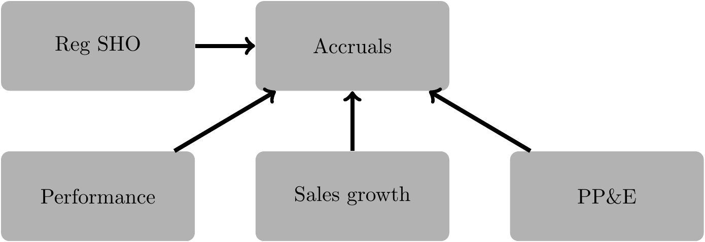
19.8.1 Discussion questions
What features of Figure 19.4 imply that we do not need to control for performance, sales, and PP&E in estimating the causal effect of Reg SHO on accruals? What is the basis for assuming these features in the causal diagram?
Black et al. (2024) report that “over 60 papers in accounting, finance, and economics report that suspension of the price tests had wide-ranging indirect effects on pilot firms, including on earnings management, investments, leverage, acquisitions, management compensation, workplace safety, and more (see Internet Appendix, Table IA-1 for a summary).” In light of the Internet Appendix of Black et al. (2024), is there any evidence that Reg SHO might plausibly have an effect on performance, sales growth, or PP&E? If so, how would Figure 19.4 need to be modified to account for these consequences? What would be the implications of these changes on the appropriate tests for estimating the causal effects of Reg SHO on accruals?
Produce a regression table like Table 19.3 and a plot like Figure 19.3, but using discretionary accruals without performance matching instead of performance-matched discretionary accruals. How do you interpret these results?
Produce a regression table and a plot like the ones in the FHK replication above, but using total accruals instead of discretionary accruals and excluding controls (so the coefficients will be simple conditional sample means). How do you interpret these results?
Suppose you had been brought in by the SEC to design a study examining the research question examined by FHK in the form of a registered report. What analyses would you conduct to try to understand the best research design? For example, how would you choose between DiD, POST, ANCOVA, and other empirical approaches? What controls would you include? How would you decide how to include controls? (For example, one could control for performance by including performance as a regressor in the model of earnings management, by matching on performance, or by including performance in the main regression specification.) How would you calculate standard errors? Discuss how your proposed empirical test differs from that of FHK. Would you have reported similar results to what FHK reported?
Suppose that FHK’s empirical analysis had produced a positive effect of Reg SHO on earnings management? Would this imply a lack of support for their hypotheses? Do you believe that publication in the Journal of Finance depended on finding a negative effect?
What implications would there have been for publication of FHK in the Journal of Finance if they had failed to find an effect of Reg SHO on earnings management?
19.9 Causal mechanisms
Black et al. (2024) suggest a number of possible causal channels through which the Reg SHO experiment could have affected the behavior of firms or third parties, including short interest, returns, price efficient, and “manager fear”. On the last of these, Black et al. (2024, p. 4) suggest that “even if the Reg SHO experiment did not actually affect short interest or returns, pilot firm managers could have feared being targeted by short sellers and taken pre-emptive actions.”
Black et al. (2024, p. 5133) argue that “if firm managers were fearful that relaxing the price tests would affect them, one might expect them to voice concerns in various ways: speaking with business news reporters; writing to the SEC when it sought public comments, or seeking meetings with SEC officials to express opposition. … We searched the business press during 2003 when the rule was proposed, in 2004 when the experiment was announced, in 2006 when the SEC proposed repeal … We found no evidence of manager opposition.”
Black et al. (2024, p. 5134) suggest that “FHK rely on the manager fear channel. They conjecture that, in response to a greater threat of short selling, pilot firms’ managers reduced earnings management to preemptively deter short sellers.”
19.9.1 Discussion questions
Do you agree with the assertion of Black et al. (2024) that “FHK rely on the manager fear channel”? What causal mechanisms are suggested in Fang et al. (2016)? What evidence do Fang et al. (2016) offer in support of these mechanisms?
Evaluate the response of Fang et al. (2019) to Black et al. (2024) as it relates to causal mechanisms?
Do you think evidence of causal mechanisms is more or less important when using a natural experiment (i.e., an experiment outside the control of the researcher that is typically analysed after it has been run) than when conducting a randomized experiment? Explain your reasoning given the various issues raised in this chapter.
19.10 Two-step regressions
Chen et al. (2018) examine the question of statistical inference when residuals from one regression are used as a dependent variable in a subsequent regression, which they refer to as “the two-step procedure”. For example, discretionary accruals measured using the Jones (1991) model are residuals from a regression of total accruals on changes in sales and PP&E. As we saw in Dechow et al. (1995), which we covered in Chapter 16, many papers examine how Jones (1991) model discretionary accruals relate to various posited incentives for earnings management.
Chen et al. (2018, p. 755) show that “the two-step procedure is likely to generate biased coefficients and t-statistics in many studies” and, drawing on the Frisch-Waugh-Lovell theorem (see Section 3.3), propose using a single regression in place of the two-step procedure. In the case of the Jones (1991) model, this would entail including the regressors from the first step in same regression as the second step and using total accruals in place of discretionary accruals as the dependent variable.
19.10.1 Discussion questions
What challenges would exist in implementing the single-regression recommendation of Chen et al. (2018) for a researcher using Kothari et al. (2005) performance-matched discretionary accruals?
Do you believe the issues raised by Chen et al. (2018) with regard to two-step procedures also apply if using randomization inference? Why or why not?
While there are two data sets calculated in Section 19.2 that are used later in the chapter, it is not necessary to run the code in this section to use the code later in the chapter, as we have provided those data sets—
sho_r3000_sampleandsho_r3000_gvkeys—as part of thefarrpackage.↩︎Note that while Bloomfield et al. (2018) discuss “\(p \leq 0.05\)”, it is more conventional to look for \(p < 0.05\), with ties effectively going to the null hypothesis; in practice, this makes no difference.↩︎
We explained the use of
pick(everything())in Chapter 13.↩︎There were multiple lists of treatment stocks, as there was a list for each exchange. These lists were updated over time as stocks changed status, a detail we gloss over for the purposes of this chapter.↩︎
We exclude non-positive values of
exchcdas these appear to be rows flagging special temporary trading statuses that create duplicate rows.↩︎In other words, we don’t need date ranges in the
gvkeystable.↩︎These data frames are derived from SAS files provided by the authors of Fang et al. (2016), as can be seen in the source code of the
farrpackage: https://go.unimelb.edu.au/ezw8.↩︎In contrast, death is one outcome where difference-in-differences analysis makes no sense for almost all individuals.↩︎
Note that the fact that the variance of \(y_t\) equals \(\frac{1}{1 - \rho^2}\)—so \(\rho = 1\) is technically problematic—and a variant of
get_outcomes()might specifye <- rnorm(periods, sd = sqrt(1 - rho^2))to hold the variance of \(y\) constant as \(\rho\) changes. Doing this does not change the tenor of the analysis, so we do not implement this here.↩︎It is not clear that the matching procedure correctly identified the group of firms considered for treatment. Kelly and Ljungqvist (2012, pp. 1386–1387) “match [control] firms [for each treatment firm] on the Fama and French (1993) pricing factors by using the Daniel et al. (1997) algorithm. Specifically, we choose as controls for terminated stock \(i\) five firms in the same size and book-to-market quintile in the preceding month of June, subject to the condition that control firms did not themselves experience a termination in the quarter before or after.” But this is the appropriate matching procedure for causal inference only if “nature” herself selected firms for consideration as treatment or control firms based on such criteria (or ones highly correlated with these).↩︎
Armstrong et al. (2022) define “quasi-experimental methods” as “methods that seek to exploit as-if random variation in observational settings”, but at other times extend this definition to include DiD.↩︎
We study Li et al. (2018) closely in Chapter 21.↩︎
The particular approach taken also implies a 50-50 split between treatment and control in expectation. We explained the use of
pick(everything())in Chapter 13.↩︎The elision of DiD with some notion of “natural experiments” seems to be a good example of the conceptual stretching discussed by Dunning (2012, p. 3). Huntington-Klein (2021) uses the term event studies to describe settings where treatment is applied during a sample period, but there is no random assignment. We avoid that term given its more specialist meaning in accounting and finance (see Chapter 13).↩︎
That is, the coefficient on \(\frac{\Delta \textit{REV}_{i,t}} {\textit{ASSET}_{i,t-1}}\) (\(\beta_2\)) from (3) in Kothari et al. (2005, p. 1263) is applied to \(\frac{(\Delta \textit{REV}_{i,t} - \Delta \textit{AR}_{i,t})}{\textit{ASSET}_{i,t-1}}\) from (4) on the same page.↩︎
We discuss winsorization and the
winsorize()function in Chapter 24.↩︎See Chapter 5 of Imbens and Rubin (2015) for details on this approach.↩︎