11 Ball and Brown (1968)
In this and the following chapter, we cover the first two winners of the Seminal Contributions to Accounting Literature Award: Ball and Brown (1968) and Beaver (1968).1
Ball and Brown (1968) won the inaugural Seminal Contribution to the Accounting Literature Award with a citation: “No other paper has been cited as often or has played so important a role in the development of accounting research during the past thirty years.” However, Philip Brown (Brown, 1989) recalled in a presentation to the 1989 JAR conference that the paper was rejected by The Accounting Review with the editor indicating a willingness to “reconsider the manuscript if Ray and I wished to cut down the empirical stuff and expand the ‘bridge’ we had tried to build between our paper and the accounting literature.” (Brown, 1989, p. 205)
According to Kothari (2001, p. 113), “Ball and Brown (1968) and Beaver (1968) heralded empirical capital markets research as it is now known.” Prior to that period, accounting research was a largely theoretical discipline focused on normative research, that is, research concerned with the “right” or “best” way to account for various events and transactions. In addition to being normative, accounting theory was largely deductive, meaning that detailed theories were derived from general principles.
Beaver (1998) identifies one approach as asking, say, “what properties should the ‘ideal’ net income have?” One answer to this question is that accounting income a period should reflect the change in the net present value of cash flows (plus cash distributions) to shareholders during the period. But other answers existed. Accounting researchers would start with a set of desired properties and use these to derive the “best” approach to accounting for depreciation of long-lived assets, inventory, or lease assets. Kothari (2001) points out that there was “little emphasis on the empirical validity” of theory.
Similar ideas still permeate the thinking of standard-setters, who purport to derive detailed accounting standards from their “conceptual frameworks”, which outline broad definitions of things such as assets and liabilities that standard-setters can supposedly use to derive the correct accounting approach in any given setting.
However, in the period since Ball and Brown (1968), these approaches have been largely discarded in academic research. A largely normative, theoretical emphasis has been replaced by a positive, empirical one.
This chapter uses Ball and Brown (2019) as a kind of reading guide to Ball and Brown (1968) before considering a replication of Ball and Brown (1968) styled on that provided by Nichols and Wahlen (2004).
The code in this chapter uses the packages listed below. Because we use several packages from the Tidyverse, we save time by using library(tidyverse) to load them in one go. For instructions on how to set up your computer to use the code found in this book, see Section 1.2. Quarto templates for the exercises below are available on GitHub.
11.1 Principal results of Ball and Brown (1968)
The first two pages of Ball and Brown (1968) address the (then) extant accounting literature. This discussion gives the impression that the (academic) conventional wisdom at that time was that accounting numbers were (more or less) meaningless (“the difference between twenty-seven tables and eight chairs”) and further research was needed to devise more meaningful accounting systems.
Arguably this notion informs the null hypothesis of Ball and Brown (1968). If accounting numbers are meaningless, then they should bear no relationship to economic decisions made by rational actors. Ball and Brown (1968) seek to test this (null) hypothesis by examining the relationship between security returns and unexpected income changes. Ball and Brown (1968) argue that “recent developments in capital theory … [justify] selecting the behavior of security prices as an operational test of usefulness.”
The evidence provided by Ball and Brown (1968) might not convince critics of the usefulness of adding chairs and tables unless the market is a rational, efficient user of a broader set of information. There are accounts for the results of Ball and Brown (1968) that do not rely on such rationality and efficiency. First, the market might react to “twenty-seven tables less eight chairs” because it does not know what it is doing. Second, the market might know that “twenty-seven tables less eight chairs” is meaningless, but has no better information to rely upon. Given the arguments they seek to address, assumptions that the market is (a) efficient and (b) has access to a rich information set beyond earnings seem implicit in the use of security returns in a test of usefulness.
Ball and Brown (2019, p. 414) identify three main results of Ball and Brown (1968): “The most fundamental result was that accounting earnings and stock returns were correlated. … Nevertheless, annual accounting earnings lacked timeliness. … After the earnings announcement month, the API (which cumulated abnormal returns) continued to drift in the same direction.”
Figure 1 of Ball and Brown (1968) depicts the data provided in Table 5 and comprises all three of the principal results flagged by Ball and Brown (2019).
The returns reported in Figure 1 of Ball and Brown (1968) are not feasible portfolios because the earnings variables used to form each portfolio at month \(-12\) are not reliably available until month \(0\) or later. Yet one can posit the existence of a mechanism (e.g., a time machine or a magical genie) that would suffice to make the portfolios notionally feasible. For example, if a genie could tell us whether earnings for the upcoming year for each firm will increase or decrease at month \(-12\), we could go long on firms expecting positive news, and go short on firms expecting negative news.2 Note that this hypothetical genie is sparing with the information she provides. For example, we might want further details on how much earnings increased or decreased, but our genie gives us just the sign of the earnings news.
Additionally, we have implicit constraints on the way we can use this information in forming portfolios. We might do better to adjust the portfolio weights according to other factors, such as size or liquidity, but the portfolios implicit in Figure 1 of Ball and Brown (1968) do not do this. Nor do the portfolios represented in Figure 1 involve any opportunity to adjust portfolio weights during the year.
In assessing the relative value of various sources of information, Ball and Brown (1968) consider three approaches to constructing portfolios, which they denote as TI, NI, and II (Ball and Brown (2019) denote II as AI and we follow this notation below). Using these metrics, Ball and Brown (1968, p. 176) conclude that “of all the information about an individual firm which becomes available during a year, one-half or more is captured in that year’s income number. … However, the annual income report does not rate highly as a timely medium, since most of its content (about 85 to 90 per cent) is captured by more prompt media which perhaps include interim reports.”3
The third principal result is shown in Table 5, where we see that the income surprise is correlated with the API to a statistically significant extent in each month up to two months after the earnings announcement.4
This result, which later become known as post-earnings announcement drift (or simply PEAD), was troubling to Ball and Brown (1968), who argue that some of it may be explained by “peak-ahead” in the measure of market income and transaction costs causing delays in trade. We study PEAD more closely in Chapter 14.
11.1.1 Discussion questions
What is the research question of Ball and Brown (1968)? Do you find the paper to be persuasive?
What do you notice about the references in Ball and Brown (1968, pp. 177–178)?
Given that “the most fundamental result” of Ball and Brown (1968) relates to an association or correlation, is it correct to say that the paper provides no evidence on causal linkages? Does this also mean that Ball and Brown (1968) is a “merely” descriptive paper according to the taxonomy of research papers outlined in Chapter 4. How might the results of Ball and Brown (1968) be represented in a causal diagram assuming that accounting information is meaningful and markets are efficient? Would an alternative causal diagram be assumed by a critic who viewed accounting information as meaningless?
Describe how Figure 1 of Ball and Brown (1968) supports each of principal results identified by Ball and Brown (2019).
Consider the causal diagrams you created above. Do the results of Ball and Brown (1968) provide more support for one causal diagram than the other.
Compare Figure 1 of Ball and Brown (2019) with Figure 1 of BB68. What is common between the two figures? What is different?
What does “less their average” mean in the title of Figure 1 of Ball and Brown (2019)? What effect does this have on the plot? (Does it make this plot different from Figure 1 of BB68? Is information lost in the process?)
Ball and Brown (2019, p. 418) say “in this replication we address two issues with the BB68 significance tests.” Do you understand the points being made here?
Ball and Brown (2019, p. 418) also say “the persistence of PEAD over time is evidence it does not constitute market inefficiency.” What do you make of this argument?
What is the minimum amount of information that our hypothetical genie needs to provide to enable formation of the portfolios underlying TI, NI, and II? What are the rules for construction of each of these portfolios?
Ball and Brown (1968) observe a ratio of NI to TI of about 0.23. What do we expect this ratio to be? Does this ratio depend on the information content of accounting information?
Consider the paragraph in Ball and Brown (2019, p. 418) beginning “an innovation in BB68 was to estimate …”. How do the discussions of these results differ between Ball and Brown (1968) and Ball and Brown (2019)?
Consider column (4) of Table 2 of Ball and Brown (2019). Is an equivalent set of numbers reported in BB68? What is the underlying investment strategy associated with this column (this need not be feasible in practice)?
Heading 6.3 of Ball and Brown (2019) is “Does ‘useful’ disprove ‘meaningless’?” Do you think that “not meaningless” implies “not useless”? Which questions (or facts) does BB68 address in these terms?
11.2 Replicating Ball and Brown (1968)
In this section, we follow Nichols and Wahlen (2004) in conducting an updated replication of Ball and Brown (1968).
We get earnings and returns data from Compustat and CRSP, respectively.
db <- dbConnect(RPostgres::Postgres(),
                bigint = "integer",
                check_interrupts = TRUE)

msf <- tbl(db, Id(schema = "crsp", table = "msf"))
msi <- tbl(db, Id(schema = "crsp", table = "msi"))
ccmxpf_lnkhist <- tbl(db, Id(schema = "crsp",
                             table = "ccmxpf_lnkhist"))
stocknames <- tbl(db, Id(schema = "crsp",
                         table = "stocknames"))

funda <- tbl(db, Id(schema = "comp", table = "funda"))
fundq <- tbl(db, Id(schema = "comp", table = "fundq"))
db <- dbConnect(duckdb::duckdb())
msf <- load_parquet(db, schema = "crsp", table = "msf")
msi <- load_parquet(db, schema = "crsp", table = "msi")
ccmxpf_lnkhist <- load_parquet(db, schema = "crsp",
table = "ccmxpf_lnkhist")
stocknames <- load_parquet(db, schema = "crsp",
table = "stocknames")
funda <- load_parquet(db, schema = "comp", table = "funda")
fundq <- load_parquet(db, schema = "comp", table = "fundq")11.2.1 Announcement dates and returns data
Getting earnings announcement dates involved significant data-collection effort for Ball and Brown (1968). Fortunately, as discussed in Ball and Brown (2019), quarterly Compustat (comp.fundq) has data on earnings announcement dates from roughly 1971 onwards. Like Ball and Brown (1968), we are only interested in fourth quarters and firms with 31 December year-ends. Because we will need to line up these dates with data from monthly CRSP (crsp.msf), we create an annc_month variable.
To compile returns for months \(t-11\) through \(t+6\) for each earnings announcement date (\(t\)) (as Ball and Brown (1968) and Nichols and Wahlen (2004) do), we will need the date values on CRSP associated with each of those months. We will create a table td_link that will provide the link between announcement events in annc_events and dates on CRSP’s monthly stock file (crsp.msf).
The first step is to create a table (crsp_dates) that orders the dates on monthly CRSP and assigns each month a corresponding “trading date” value (td), which is 1 for the first month, 2 for the second month, and so on. Because the date values on crsp.msf line up with the date values on crsp.msi, we can use the latter (much smaller) table.
crsp_dates <-
  msi |>
  select(date) |>
  window_order(date) |>
  mutate(td = row_number()) |>
  mutate(month = as.Date(floor_date(date, unit = "month")))

crsp_dates |> collect(n = 10)
# A tibble: 10 × 3
date td month
<date> <dbl> <date>
1 1925-12-31 1 1925-12-01
2 1926-01-30 2 1926-01-01
3 1926-02-27 3 1926-02-01
4 1926-03-31 4 1926-03-01
5 1926-04-30 5 1926-04-01
6 1926-05-28 6 1926-05-01
7 1926-06-30 7 1926-06-01
8 1926-07-31 8 1926-07-01
9 1926-08-31 9 1926-08-01
10 1926-09-30 10 1926-09-01We want to construct a table that allows us to link earnings announcements (annc_events) with returns from crsp.msf Because we are only interested in months where returns are available, we can obtain the set of potential announcement months from crsp_dates. The table annc_months has each value of annc_month and its corresponding annc_td from crsp_dates, along with the boundaries of the window that contains all values of td within the range \((t - 11, t+ 6)\), where \(t\) is the announcement month.
annc_months <-
  crsp_dates |>
  select(month, td) |>
  rename(annc_month = month, annc_td = td) |>
  mutate(start_td = annc_td - 11L,
         end_td = annc_td + 6L)

annc_months |> collect(n = 10)
# A tibble: 10 × 4
annc_month annc_td start_td end_td
<date> <dbl> <dbl> <dbl>
1 1925-12-01 1 -10 7
2 1926-01-01 2 -9 8
3 1926-02-01 3 -8 9
4 1926-03-01 4 -7 10
5 1926-04-01 5 -6 11
6 1926-05-01 6 -5 12
7 1926-06-01 7 -4 13
8 1926-07-01 8 -3 14
9 1926-08-01 9 -2 15
10 1926-09-01 10 -1 16We can then join annc_months with crsp_dates to create the table td_link.
td_link <-
  crsp_dates |>
  inner_join(annc_months, join_by(between(td, start_td, end_td))) |>
  mutate(rel_td = td - annc_td) |>
  select(annc_month, rel_td, date)
Here are the data for one annc_month:
# A tibble: 18 × 3
   annc_month rel_td date
   <date>      <dbl> <date>
 1 2001-04-01      6 2001-10-31
 2 2001-04-01      5 2001-09-28
 3 2001-04-01      4 2001-08-31
 4 2001-04-01      3 2001-07-31
 5 2001-04-01      2 2001-06-29
 6 2001-04-01      1 2001-05-31
 7 2001-04-01      0 2001-04-30
 8 2001-04-01     -1 2001-03-30
 9 2001-04-01     -2 2001-02-28
10 2001-04-01     -3 2001-01-31
11 2001-04-01     -4 2000-12-29
12 2001-04-01     -5 2000-11-30
13 2001-04-01     -6 2000-10-31
14 2001-04-01     -7 2000-09-29
15 2001-04-01     -8 2000-08-31
16 2001-04-01     -9 2000-07-31
17 2001-04-01    -10 2000-06-30
18 2001-04-01    -11 2000-05-31
We use ccm_link (as used in Chapter 7) to connect earnings announcement dates on Compustat with returns from CRSP.
Nichols and Wahlen (2004) focus on firms listed on NYSE, AMEX, and NASDAQ, which correspond to firms with exchcd values of 1, 2, and 3, respectively. The value of exchcd for each firm at each point in time is found on crsp.stocknames. Following Nichols and Wahlen (2004), we get data on fiscal years from 1988 to 2002 (2004, p. 270).
rets_all <-
  annc_events |>
  inner_join(td_link, by = "annc_month") |>
  inner_join(ccm_link, by = "gvkey") |>
  filter(annc_month >= linkdt,
         annc_month <= linkenddt | is.na(linkenddt)) |>
  inner_join(msf, by = c("permno", "date")) |>
  inner_join(stocknames, by = "permno") |>
  filter(between(date, namedt, nameenddt),
         exchcd %in% c(1, 2, 3)) |>
  select(gvkey, datadate, rel_td, permno, date, ret) |>
  filter(between(year(datadate), 1987L, 2002L)) |>
  collect()
To keep things straightforward, we focus on firms that have returns for each month in the \((t - 11, t+ 6)\) window and the table full_panel identifies these firms.
Note that, unlike other early papers (e.g., Beaver, 1968; Fama et al., 1969), Ball and Brown (1968) do not exclude observations due to known confounding events.5
11.2.2 Data on size-portfolio returns
Ball and Brown (1968) focus on abnormal returns and estimate a market model with firm-specific coefficients as the basis for estimating residual returns, which they denote API. The use of residuals from a market model addresses a concern about cross-sectional correlation that would arise if raw returns were used. Ball and Brown (1968) note that about \(10\%\) of returns are due to industry factors, but conclude that the likely impact of this on inference is likely to be small.
In contrast, Nichols and Wahlen (2004) use size-adjusted returns as their measure of abnormal returns. To calculate size-adjusted returns, we get two kinds of data from the website of Ken French (as seen in Chapter 9).
First, we get data on size-decile returns. Ken French’s website supplies a comma-delimited text file containing monthly and annual data for value-weighted and equal-weighted portfolio returns.
t <- "Portfolios_Formed_on_ME_CSV.zip"
url <- str_c("http://mba.tuck.dartmouth.edu",
             "/pages/faculty/ken.french/ftp/",
             "Portfolios_Formed_on_ME_CSV.zip")
if (!file.exists(t)) download.file(url, t)
From inspection of the downloaded text file, we observe that there are several data sets in this file. We want monthly returns and will extract both value-weighted and equal-weighted data. We see that the equal-weighted returns begin with a row starting with text Equal Weight Returns -- Monthly and end a few rows before a row starting with text Value Weight Returns -- Annual.
# Determine breakpoints (lines) for different tables
temp <- read_lines(t)
vw_start <- str_which(temp, "^\\s+Value Weight Returns -- Monthly")
vw_end <- str_which(temp, "^\\s+Equal Weight Returns -- Monthly") - 4

ew_start <- str_which(temp, "^\\s+Equal Weight Returns -- Monthly")
ew_end <- str_which(temp, "^\\s+Value Weight Returns -- Annual") - 4
Having identified these separating rows, we can use the following function to read in the data set and organize the associated data tables appropriately. Note that NA values are represented as -99.99 in the text files and that the dates have a form yyyymm that we convert to dates of form yyyy-mm-01, which we call month.
While the original data come in a “wide” format with returns at every fifth percentile, we rearrange the data into a “long” format, retain only the deciles (i.e., every tenth percentile), and rename the decile labels from Lo 10, Dec 2, …, Dec 9, and Hi 10 to 1, 2, …, 9, and 10.
read_data <- function(start, end) {

  Sys.setenv(VROOM_CONNECTION_SIZE = 500000)

  fix_names <- function(names) {
    str_replace_all(names, "^$", "date")
  }

  read_csv(t, skip = start, n_max = end - start,
           na = "-99.99",
           name_repair = fix_names,
           show_col_types = FALSE) |>
    mutate(month = ymd(str_c(date, "01"))) |>
    select(-date) |>
    pivot_longer(names_to = "quantile",
                 values_to = "ret",
                 cols = -month) |>
    mutate(ret = ret / 100,
           decile = case_when(quantile == "Hi 10" ~ "10",
                              quantile == "Lo 10" ~ "1",
                              str_detect(quantile, "^Dec ") ~
                                sub("^Dec ", "", quantile)),
           decile = as.integer(decile)) |>
    filter(!is.na(decile)) |>
    select(-quantile)
}
Now we can apply this function to extract the relevant data, which we combine into a single data frame size_rets.
vw_rets <-
  read_data(vw_start, vw_end) |>
  rename(vw_ret = ret)

ew_rets <-
  read_data(ew_start, ew_end) |>
  rename(ew_ret = ret)

size_rets <-
  ew_rets |>
  inner_join(vw_rets, by = c("month", "decile")) |>
  select(month, decile, everything())

size_rets
# A tibble: 11,770 × 4
month decile ew_ret vw_ret
<date> <int> <dbl> <dbl>
1 1926-07-01 1 -0.0142 -0.0012
2 1926-07-01 2 0.0029 0.0052
3 1926-07-01 3 -0.0015 -0.0005
4 1926-07-01 4 0.0088 0.0082
5 1926-07-01 5 0.0145 0.0139
6 1926-07-01 6 0.0185 0.0189
7 1926-07-01 7 0.0163 0.0162
8 1926-07-01 8 0.0138 0.0129
9 1926-07-01 9 0.0338 0.0353
10 1926-07-01 10 0.0329 0.0371
# ℹ 11,760 more rowsThe second set of data we need to get from Ken French’s website is data on the cut-offs we will use in assigning firms to decile portfolios in calculating size-adjusted returns.
Again the original data come in a “wide” format with cut-offs at every fifth percentile, so again we rearrange the data into a “long” format, retain only the deciles (i.e., every tenth percentile), and rename the decile labels from p10, p20, …, p90, and p100, to 1, 2, …, 9, and 10.6 Also, we are only interested in the cut-offs for December in each year and use filter() to retain only these.
me_breakpoints_raw <-
  read_csv(t, skip = 1,
           col_names = c("month", "n",
                         str_c("p", seq(from = 5, to = 100, by = 5))),
           col_types = "c",
           n_max = str_which(temp, "^Copyright") - 3) |>
  mutate(month = ymd(str_c(month, "01"))) |>
  select(-ends_with("5"), -n) |>
  pivot_longer(cols = - month,
               names_to = "decile",
               values_to = "cutoff") |>
  mutate(decile = str_replace(decile, "^p(.*)0$", "\\1")) |>
  mutate(decile = as.integer(decile))
Finally, we organize the data to facilitate their use in joining with other data. Specifically, we create variables for the range of values covered by each decile (from me_min to me_max). We specify the minimum value for the first decile as zero and the maximum value for the tenth decile to infinity (Inf).
To assign stocks to size deciles, we collect data on market capitalization from crsp.msf
We can compare market capitalization for each firm-year with the cut-offs in me_breakpoints to obtain its decile assignment.
me_decile_assignments <-
  me_values |>
  inner_join(me_breakpoints,
             join_by(month, mktcap >= me_min, mktcap < me_max)) |>
  mutate(year = as.integer(year(date)) + 1L) |>
  select(permno, year, decile)
11.2.3 Earnings news variables
The main issue that Ball and Brown (1968) need to tackle regarding earnings news is one that persists in accounting research today: how does one measure the unanticipated component of income? Alternatively, how does one estimate earnings expectations of the “market”?
Ball and Brown (1968) use two measures of expected earnings. The first is a naive model that simply “predicts that income will be the same for this year as for the last” (1968, p. 163). The second uses a model that estimates a relationship between the changes in income for a firm and for the market and then applies that relationship to the contemporaneous observation of the market’s income. Note that this is an interesting variable: the equity market does not know the income for all firms at the start of the year. So the expectation is conditional with respect to a rather peculiar information set. In effect, the question is whether, given information about the market’s earnings and market returns, information about accounting earnings helps predict the unexpected portion of earnings. In any case, the main results (see the famous Figure 1) are robust to the choice of the expectations model.
news <-
  funda |>
  filter(indfmt == "INDL", datafmt == "STD",
         consol == "C", popsrc == "D") |>
  filter(fyr == 12) |>
  group_by(gvkey) |>
  window_order(datadate) |>
  mutate(lag_ibc = lag(ibc),
         lag_oancf = lag(oancf),
         lag_at = lag(at),
         lag_fyear = lag(fyear)) |>
  ungroup() |>
  filter(between(fyear, 1987, 2002),
         lag_fyear + 1 == fyear) |>
  mutate(earn_chg = if_else(lag_at > 0, (ibc - lag_ibc) / lag_at, NA),
         cfo_chg = if_else(lag_at > 0, (oancf - lag_oancf) / lag_at, NA),
         earn_gn = earn_chg > 0,
         cfo_gn = cfo_chg > 0) |>
  filter(!is.na(cfo_gn), !is.na(earn_gn)) |>
  select(gvkey, datadate, earn_chg, cfo_chg, earn_gn, cfo_gn) |>
  group_by(datadate) |>
  mutate(earn_decile = ntile(earn_chg, 10),
         cfo_decile = ntile(cfo_chg, 10)) |>
  ungroup() |>
  collect()
11.2.4 Figure 1 of Ball and Brown (1968)
We can now merge our data tables to create the data set we can use to make variants of Figure 1 of Ball and Brown (1968).
merged <-
news |>
mutate(year = year(datadate)) |>
inner_join(rets, by = c("gvkey", "datadate")) |>
inner_join(me_decile_assignments, by = c("permno", "year")) |>
mutate(month = floor_date(date, unit = "month")) |>
inner_join(size_rets, by = c("decile", "month")) |>
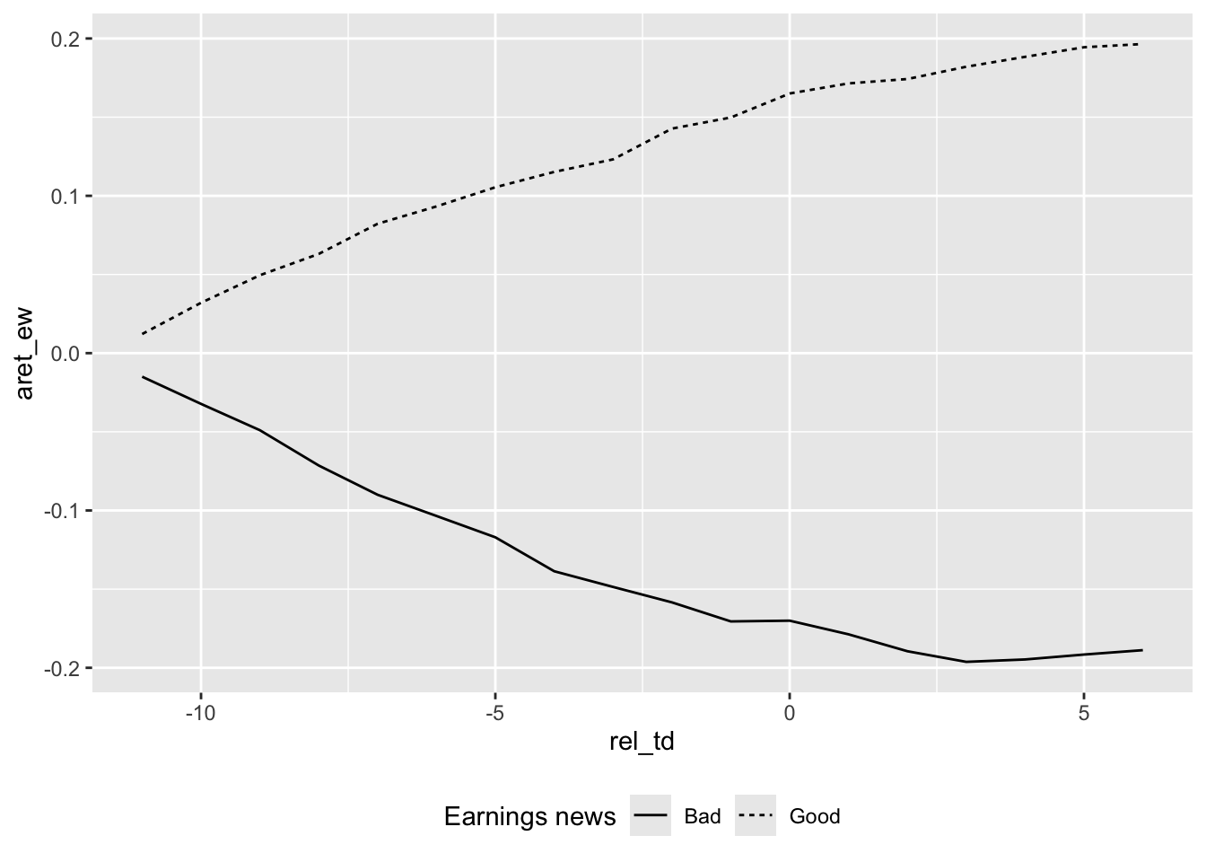
select(-permno, -month)To prepare the data for our plot, we first need to accumulate returns over time for each firm. We then need to aggregate these returns by portfolio (here earn_gn) and relative trading date (rel_td). Following Ball and Brown (1968), we calculate abnormal returns by subtracting market returns from the portfolio returns. Here we calculate measures using both equal-weighted (ew_ret) and value-weighted (vw_ret) market returns.
plot_data <-
  merged |>
  filter(!is.na(ret)) |>
  group_by(gvkey, datadate) |>
  arrange(rel_td) |>
  mutate(across(ends_with("ret"),
                \(x) cumprod(1 + x))) |>
  group_by(rel_td, earn_gn) |>
  summarize(across(ends_with("ret"),
                   \(x) mean(x, na.rm = TRUE)),
            .groups = "drop") |>
  mutate(aret_ew = ret - ew_ret, aret_vw = ret - vw_ret)
Figure 1 of Ball and Brown (1968) confirms that a picture is worth a thousand words. We produce our analogue of Figure 1 in Figure 11.1.
11.2.5 Exercises
- From the data below, we see that the upper bound for the tenth decile is about US$544 billion. How can we reconcile this with the existence of firms with market capitalizations over US$1 trillion? Bonus: Using data from
crsp.msf, identify the firm whose market capitalization was US$544 billion in December 2020? (Hint: For the bonus question, you can add afilter()to code in the template to obtain the answer. Why do we need to group bypermco, notpermno, to find the answer?)
me_breakpoints_raw |>
  filter(month == "2020-12-01")
# A tibble: 10 × 3
month decile cutoff
<date> <int> <dbl>
1 2020-12-01 1 327.
2 2020-12-01 2 756.
3 2020-12-01 3 1439.
4 2020-12-01 4 2447.
5 2020-12-01 5 3655.
6 2020-12-01 6 5544
7 2020-12-01 7 9656.
8 2020-12-01 8 17056.
9 2020-12-01 9 37006.
10 2020-12-01 10 543615.To keep things straightforward, we focused on firms that have returns for each month in the \((t - 11, t+ 6)\) window. Can you tell what approach Nichols and Wahlen (2004) took with regard to this issue?
Table 2 of Nichols and Wahlen (2004) measures cumulative abnormal returns as the “cumulative raw return minus cumulative size decile portfolio to which the firm begins.” Apart from the use of a size-decile portfolio rather than some other market index, how does this measure differ from the Abnormal Performance Index (API) defined on p.168 of Ball and Brown (1968)? Adjust the measure depicted in the replication of Figure 1 to more closely reflect the API definition used in Ball and Brown (1968) (but retaining the size-decile as the benchmark). Does this tweak significantly affect the results? Which approach seems most appropriate? That of Nichols and Wahlen (2004) or that of Ball and Brown (1968)?
Create an alternative version of Figure 11.1 using the sign of “news” about cash flows in the place of income news. Do your results broadly line up with those in Panel A of Figure 2 of Nichols and Wahlen (2004)? Do these results imply that accounting income is inherently more informative than cash flows from operations? Why or why not?
Create an alternative version of the figure above focused on the extreme earnings deciles in place of the good-bad news dichotomy. Do your results broadly line up with those in Panel B of Figure 2 of Nichols and Wahlen (2004)?
Calculate AI by year following the formula on p. 175 of Ball and Brown (1968) (there denoted as \(II_0\)). You may find it helpful to start with the code producing
plot_dataabove. You may also find it helpful to use the functionpivot_widerto get information about portfolios in each year into a single row. Note that you will only be interested in rows at \(t = 0\) (e.g.,filter(rel_td == 0)).Calculate NI by year following the formula on p. 175 of Ball and Brown (1968) (there denoted as \(NI_0\)). Note that you will only be interested in rows at \(t = 0\) (e.g.,
filter(rel_td == 0)).Using the data on NI and AI from above, create a plot of \(AI/NI\) like that in Figure 2 of Ball and Brown (2019). Do you observe similar results to those shown in Figure 2 of Ball and Brown (2019)?
The list of winners can be found at https://go.unimelb.edu.au/yzw8.↩︎
Actually, because the lines of Figure 1 represent abnormal returns, the associated portfolios involve going long or short in each of a group of stocks and short or long in a broader market index at the same time.↩︎
For more on the “apparent paradox” discussed on p.176, see Leftwich and Zmijewski (1994).↩︎
There are some months where this does not hold, but the statement is broadly true.↩︎
This issue seems related to that discussed on p.164, where Ball and Brown (1968) state “our prediction [is] that, or certain months around the report dates, the expected values of the \(v_j\)’s are nonzero.” They defend the absence of an exclusion period on the basis that there is a low, observed autocorrelation in the \(v_j\)’s, and in no case was the stock return regression fitted over less than 100 observations.” (Ball and Brown, 1968, p. 164). But note that the basis for assuming that the expected value of \(v_j\) is nonzero in any given month is much less clear in this setting than it was in Fama et al. (1969). Given that a company will announce earnings in a particular month, this announcement could be either good or bad news, so the expected abnormal return seems likely to be zero.↩︎
Unlike the data set on returns above, there are no column labels in this data set and we are making those ourselves here.↩︎